Note
Go to the end to download the full example code.
06 Surrogate Models with Machine Learning#
This example demonstrates how to build machine-learning surrogate models to predict CFAST outputs instantly instead of running full simulations.
We predict the maximum Target Surface Temperature (TRGSURT) reached during
a CFAST simulation of a target Device, using various fire
parameters (heat of combustion, radiative fraction, soot yield and target z position)
as inputs. Several machine learning models will be evaluated including linear
regression, polynomial regression, gradient boosting, random forest, and a simple
neural network.
Step 1: Import Required Libraries#
import matplotlib.pyplot as plt
import numpy as np
import seaborn as sns
import torch
import torch.nn as nn
import torch.optim as optim
from sklearn.ensemble import GradientBoostingRegressor, RandomForestRegressor
from sklearn.linear_model import LinearRegression
from sklearn.metrics import mean_squared_error, r2_score
from sklearn.model_selection import train_test_split
from sklearn.pipeline import Pipeline
from sklearn.preprocessing import PolynomialFeatures, StandardScaler
from torch.utils.data import DataLoader, TensorDataset

from pycfast.datasets import load_sp_ast_diesel_1p1
from pycfast.parsers import parse_cfast_file

plt.style.use("seaborn-v0_8-whitegrid")
Step 2: Load Base Model and Run Baseline#
We use parse_cfast_file to load the base model.
model = parse_cfast_file("data/SP_AST_Diesel_1p1.in")
The parsed model is displayed below.
print(model.summary())
Model: SP_AST_Diesel_1p1_parsed.in
Simulation: 'CFAST Simulation' (1800s)

Components:
  Material Properties (1):
    Material 'STEELSHT' (Steel Plain Carbon (1/16 in)): k=48.0, ρ=7854.0, c=0.559, t=0.0015, ε=0.9
  Compartment (1):
    Compartment 'Compartment 1': 100.0x100.0x100.0 m, volume: 1000000.00 m³ (ceiling: OFF, wall: OFF, floor: OFF)
  Wall Vents (4):
    Wall Vent 'WallVent_1': Compartment 1 ↔ OUTSIDE, 100.0x100.0 m, bottom: 0.0 m
    Wall Vent 'WallVent_2': Compartment 1 ↔ OUTSIDE, 100.0x100.0 m, bottom: 0.0 m
    Wall Vent 'WallVent_3': Compartment 1 ↔ OUTSIDE, 100.0x100.0 m, bottom: 0.0 m
    Wall Vent 'WallVent_4': Compartment 1 ↔ OUTSIDE, 100.0x100.0 m, bottom: 0.0 m
  Fire (1):
    Fire 'n-Decane Test 1' (n-Decane Test 1_Fire) in 'Compartment 1' at (50, 50) (peak: 2 kW, duration: 27min, χr: 0.35)
  Device (5):
    Target 'Targ 1' (PLATE) in 'Compartment 1' at (50, 50, 1.45) (material: STEELSHT, depth: 0.00075m)
    Target 'Targ 2' (PLATE) in 'Compartment 1' at (50, 50, 2.45) (material: STEELSHT, depth: 0.00075m)
    Target 'Targ 3' (PLATE) in 'Compartment 1' at (50, 50, 3.45) (material: STEELSHT, depth: 0.00075m)
    Target 'Targ 4' (PLATE) in 'Compartment 1' at (50, 50, 4.45) (material: STEELSHT, depth: 0.00075m)
    Target 'Targ 5' (PLATE) in 'Compartment 1' at (50, 50, 5.45) (material: STEELSHT, depth: 0.00075m)
We use run to get baseline results
baseline_results = model.run()

print(f"Baseline TRGSURT max: {baseline_results['devices']['TRGSURT_1'].max():.2f} °C")
print("Current fire parameters:")
print(f"Heat of combustion: {model.fires[0].heat_of_combustion} kJ/kg")
print(f"Radiative fraction: {model.fires[0].radiative_fraction}")
print(f"Soot yield: {model.fires[0].data_table[0][5]}")
Baseline TRGSURT max: 920.10 °C
Current fire parameters:
Heat of combustion: 50000.0 kJ/kg
Radiative fraction: 0.35
Soot yield: 0.05
Step 3: Load Pre-computed Training Data#
Instead of running 5000 CFAST simulations (which can take hours),
we load a precomputed dataset that is included with pycfast using
load_sp_ast_diesel_1p1.
The data was generated once with Sobol quasi-random sampling across the parameter space (see the module docstring for full details).
training_data = load_sp_ast_diesel_1p1()
The dataset contains the following columns:
The target variable is max_trgsurt which is the maximum surface temperature of the target device during the simulation. The input parameters are heat_of_combustion, radiative_fraction, soot_yield, and target_location_z.
Step 4: Quick Data Exploration#
Before training surrogate models, it’s helpful to understand the relationships between the input parameters and the target variable. We can compute correlation coefficients to see which parameters have the strongest influence on TRGSURT.
input_params = [
    "heat_of_combustion",
    "radiative_fraction",
    "soot_yield",
    "target_location_z",
]
correlations = training_data[input_params].corrwith(training_data["max_trgsurt"])

print("Parameter correlations with TRGSURT:")
for param, corr in correlations.abs().sort_values(ascending=False).items():
    direction = "+" if correlations[param] > 0 else "-"
    print(f"{param}: {direction}{corr:.3f}")
Parameter correlations with TRGSURT:
target_location_z: -0.939
radiative_fraction: +0.129
soot_yield: -0.001
heat_of_combustion: +0.001
We can also visualize the correlation matrix to see how the input parameters correlate with each other and with the target variable.
fig, ax = plt.subplots(1, 1, figsize=(8, 6))
sns.heatmap(training_data.corr(), annot=True, cmap="coolwarm", center=0, ax=ax)
plt.title("Parameter Correlation Matrix")
plt.tight_layout()
plt.show()
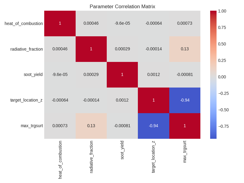
The correlation analysis shows that target height (z-axis position) has the strongest negative correlation with TRGSURT, which underscores how strongly radiative heat transfer drives target surface temperatures. This makes physical sense since the farther the target device is from the fire source, the lower the surface temperature it experiences. Radiative fraction shows the second strongest correlation, showing the importance of radiative heat transfer in determining target surface temperatures in fire scenarios.
Step 5: Train Surrogate Models#
Now we can train different surrogate models to predict TRGSURT based on the input parameters. We’ll evaluate the performance of each model using R² and RMSE metrics on a held-out test set. First, we split the data into training and testing sets.
X = training_data[input_params].values
y = training_data["max_trgsurt"].values
X_train, X_test, y_train, y_test = train_test_split(
    X, y, test_size=0.2, random_state=42
)
Next, we define and train several machine learning models.
Prepare models and evaluate their performance:
Linear Regression
Polynomial Regression
models["Polynomial"] = Pipeline(
    [
        ("scaler", StandardScaler()),
        ("poly", PolynomialFeatures(degree=2, include_bias=False)),
        ("regressor", LinearRegression()),
    ]
)
models["Polynomial"].fit(X_train, y_train)
y_pred = models["Polynomial"].predict(X_test)
metrics["Polynomial"] = {
    "R²": r2_score(y_test, y_pred),
    "RMSE": np.sqrt(mean_squared_error(y_test, y_pred)),
}
Gradient Boosting
models["Gradient Boosting"] = Pipeline(
    [
        ("scaler", StandardScaler()),
        ("regressor", GradientBoostingRegressor(n_estimators=100, random_state=42)),
    ]
)
models["Gradient Boosting"].fit(X_train, y_train)
y_pred = models["Gradient Boosting"].predict(X_test)
metrics["Gradient Boosting"] = {
    "R²": r2_score(y_test, y_pred),
    "RMSE": np.sqrt(mean_squared_error(y_test, y_pred)),
}
Random Forest
models["Random Forest"] = Pipeline(
    [
        ("scaler", StandardScaler()),
        ("regressor", RandomForestRegressor(n_estimators=100, random_state=42)),
    ]
)
models["Random Forest"].fit(X_train, y_train)
y_pred = models["Random Forest"].predict(X_test)
metrics["Random Forest"] = {
    "R²": r2_score(y_test, y_pred),
    "RMSE": np.sqrt(mean_squared_error(y_test, y_pred)),
}
Neural net model
class SimpleNN(nn.Module):
    def __init__(self, input_size):
        super().__init__()
        self.net = nn.Sequential(
            nn.Linear(input_size, 16),
            nn.ReLU(),
            nn.Linear(16, 16),
            nn.ReLU(),
            nn.Linear(16, 1),
        )

    def forward(self, x):
        return self.net(x)


scaler_nn = StandardScaler()
X_train_scaled = scaler_nn.fit_transform(X_train)
X_test_scaled = scaler_nn.transform(X_test)

y_scaler = StandardScaler()
y_train_scaled = y_scaler.fit_transform(y_train.reshape(-1, 1)).flatten()

X_train_tensor = torch.FloatTensor(X_train_scaled)
y_train_tensor = torch.FloatTensor(y_train_scaled).reshape(-1, 1)
X_test_tensor = torch.FloatTensor(X_test_scaled)

val_fraction = 0.2
n_val = int(len(X_train_tensor) * val_fraction)
X_val_tensor = X_train_tensor[:n_val]
y_val_tensor = y_train_tensor[:n_val]
X_tr_tensor = X_train_tensor[n_val:]
y_tr_tensor = y_train_tensor[n_val:]

train_dataset = TensorDataset(X_tr_tensor, y_tr_tensor)
val_dataset = TensorDataset(X_val_tensor, y_val_tensor)

train_loader = DataLoader(train_dataset, batch_size=16, shuffle=True)
val_loader = DataLoader(val_dataset, batch_size=256, shuffle=False)

model_nn = SimpleNN(X_train.shape[1])
criterion = nn.MSELoss()
optimizer = optim.Adam(model_nn.parameters(), lr=0.001, weight_decay=1e-5)
scheduler = optim.lr_scheduler.ReduceLROnPlateau(
    optimizer, mode="min", factor=0.5, patience=10
)

best_val_loss = float("inf")
patience = 20
patience_counter = 0
best_state = None

history = {"train": [], "val": []}

for epoch in range(1000):
    model_nn.train()
    train_loss = 0.0
    for batch_X, batch_y in train_loader:
        optimizer.zero_grad()
        outputs = model_nn(batch_X)
        loss = criterion(outputs, batch_y)
        loss.backward()
        torch.nn.utils.clip_grad_norm_(model_nn.parameters(), max_norm=1.0)
        optimizer.step()
        train_loss += loss.item()
    train_loss /= len(train_loader)

    model_nn.eval()
    with torch.no_grad():
        val_loss = 0.0
        for batch_X, batch_y in val_loader:
            outputs = model_nn(batch_X)
            val_loss += criterion(outputs, batch_y).item()
        val_loss /= len(val_loader)

    scheduler.step(val_loss)

    history["train"].append(train_loss)
    history["val"].append(val_loss)

    if epoch % 40 == 0:
        print(
            f"Epoch {epoch}, Train Loss: {train_loss:.6f}, Val Loss: {val_loss:.6f}, LR: {optimizer.param_groups[0]['lr']:.6f}"
        )

    if val_loss < best_val_loss:
        best_val_loss = val_loss
        best_state = {k: v.clone() for k, v in model_nn.state_dict().items()}
        patience_counter = 0
    else:
        patience_counter += 1
        if patience_counter >= patience:
            print(f"Early stopping at epoch {epoch + 1}")
            break

if best_state:
    model_nn.load_state_dict(best_state)

model_nn.eval()
with torch.no_grad():
    y_pred_nn_scaled = model_nn(X_test_tensor).cpu().numpy()
    y_pred_nn = y_scaler.inverse_transform(y_pred_nn_scaled).flatten()

models["Neural Network"] = {
    "model": model_nn,
    "scaler": scaler_nn,
    "y_scaler": y_scaler,
}

metrics["Neural Network"] = {
    "R²": r2_score(y_test, y_pred_nn),
    "RMSE": np.sqrt(mean_squared_error(y_test, y_pred_nn)),
}
Epoch 0, Train Loss: 0.607825, Val Loss: 0.146404, LR: 0.001000
Epoch 40, Train Loss: 0.000390, Val Loss: 0.000303, LR: 0.001000
Epoch 80, Train Loss: 0.000140, Val Loss: 0.000124, LR: 0.000500
Epoch 120, Train Loss: 0.000106, Val Loss: 0.000113, LR: 0.000250
Epoch 160, Train Loss: 0.000083, Val Loss: 0.000096, LR: 0.000125
Epoch 200, Train Loss: 0.000068, Val Loss: 0.000072, LR: 0.000063
Epoch 240, Train Loss: 0.000063, Val Loss: 0.000066, LR: 0.000016
Early stopping at epoch 254
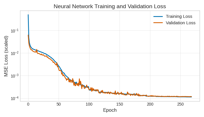
Plotting the training history shows that the model is learning well without overfitting.
plt.figure(figsize=(7, 4))
plt.plot(history["train"], label="Training Loss", color="#0072B2", linewidth=2)
plt.plot(history["val"], label="Validation Loss", color="#D55E00", linewidth=2)
plt.xlabel("Epoch", fontsize=12)
plt.ylabel("MSE Loss (scaled)", fontsize=12)
plt.title("Neural Network Training and Validation Loss", fontsize=14)
plt.yscale("log")
plt.legend(fontsize=11)
plt.grid(True, alpha=0.4)

min_val_epoch = np.argmin(history["val"])
min_val_loss = history["val"][min_val_epoch]

plt.tight_layout()
plt.show()
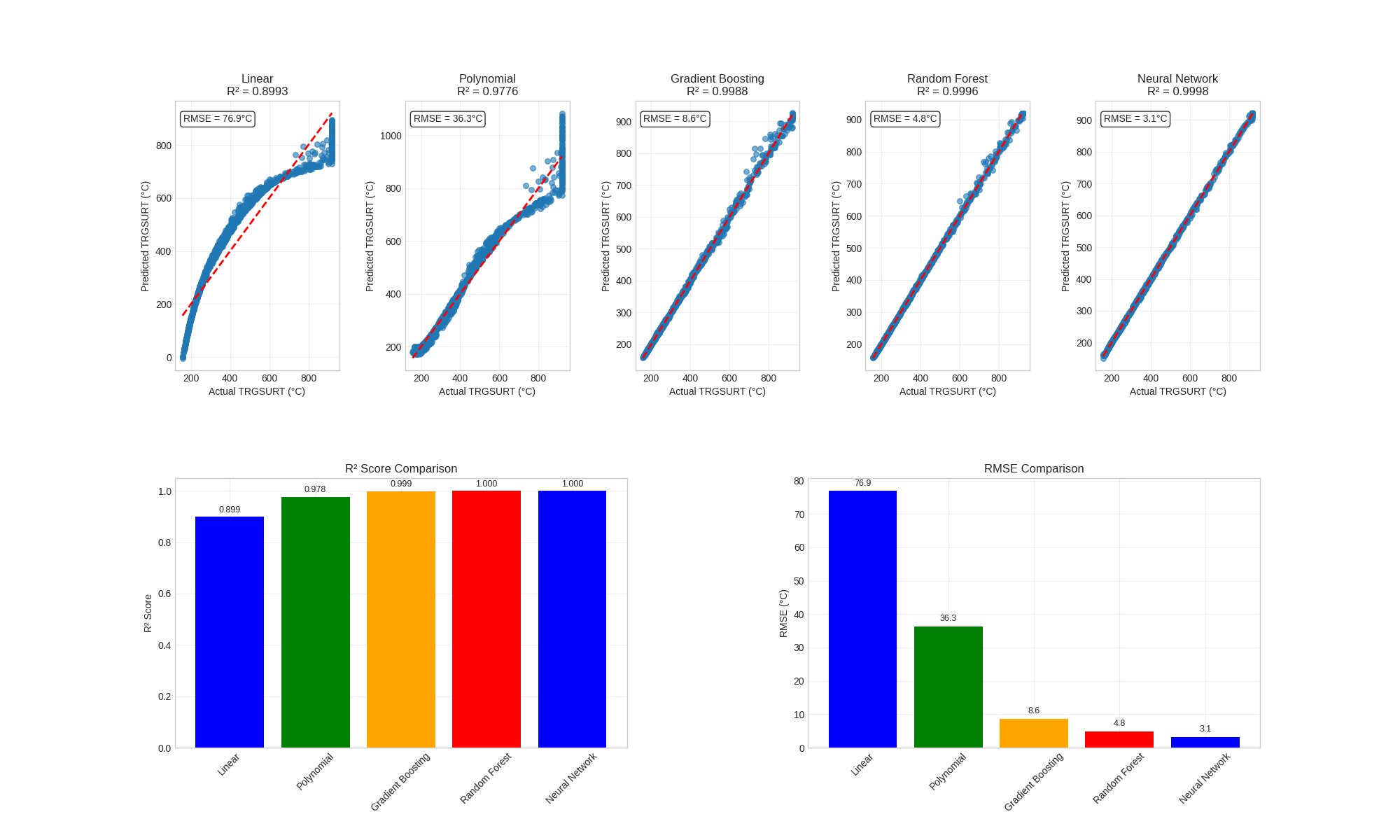
Step 6: Evaluate and Compare Models#
Now that we have trained several surrogate models, we can evaluate their performance on the test set and compare their predictions against the actual CFAST simulation results. Below is a summary of the performance metrics for each model.
for name, metric in metrics.items():
    print(f"{name}: R² = {metric['R²']:.4f}, RMSE = {metric['RMSE']:.2f} °C")

best_model = max(metrics.keys(), key=lambda k: metrics[k]["R²"])
print(f"\nBest model: {best_model} (R² = {metrics[best_model]['R²']:.4f})")
Linear: R² = 0.8993, RMSE = 76.91 °C
Polynomial: R² = 0.9776, RMSE = 36.30 °C
Gradient Boosting: R² = 0.9986, RMSE = 8.92 °C
Random Forest: R² = 0.9996, RMSE = 4.75 °C
Neural Network: R² = 0.9999, RMSE = 2.21 °C

Best model: Neural Network (R² = 0.9999)
We can also visualize the predictions of each model against the actual values to see how well they match.
model_names = list(metrics.keys())
n_models = len(model_names)

fig = plt.figure(figsize=(20, 12))

for i, model_name in enumerate(model_names):
    ax = plt.subplot(2, n_models, i + 1)

    if model_name == "Neural Network":
        model_obj = models[model_name]
        model_obj["model"].eval()
        with torch.no_grad():
            y_pred_scaled = model_obj["model"](X_test_tensor).numpy()
            y_pred = model_obj["y_scaler"].inverse_transform(y_pred_scaled).flatten()
    else:
        y_pred = models[model_name].predict(X_test)

    ax.scatter(y_test, y_pred, alpha=0.6, s=30)
    min_val, max_val = y_test.min(), y_test.max()
    ax.plot([min_val, max_val], [min_val, max_val], "r--", linewidth=2)
    ax.set_xlabel("Actual TRGSURT (°C)")
    ax.set_ylabel("Predicted TRGSURT (°C)")
    ax.set_title(f"{model_name}\nR² = {metrics[model_name]['R²']:.4f}")
    ax.grid(True, alpha=0.3)

    ax.text(
        0.05,
        0.95,
        f"RMSE = {metrics[model_name]['RMSE']:.1f}°C",
        transform=ax.transAxes,
        verticalalignment="top",
        bbox={"boxstyle": "round", "facecolor": "white", "alpha": 0.8},
    )

ax_r2 = plt.subplot(2, 2, 3)
r2_scores = [metrics[m]["R²"] for m in model_names]
colors = ["blue", "green", "orange", "red"][: len(model_names)]

bars = ax_r2.bar(model_names, r2_scores, color=colors)
ax_r2.set_ylabel("R² Score")
ax_r2.set_title("R² Score Comparison")
ax_r2.tick_params(axis="x", rotation=45)
ax_r2.grid(True, alpha=0.3)

for bar, score in zip(bars, r2_scores, strict=False):
    height = bar.get_height()
    ax_r2.text(
        bar.get_x() + bar.get_width() / 2.0,
        height + 0.01,
        f"{score:.3f}",
        ha="center",
        va="bottom",
        fontsize=9,
    )

ax_rmse = plt.subplot(2, 2, 4)
rmse_scores = [metrics[m]["RMSE"] for m in model_names]

bars = ax_rmse.bar(model_names, rmse_scores, color=colors)
ax_rmse.set_ylabel("RMSE (°C)")
ax_rmse.set_title("RMSE Comparison")
ax_rmse.tick_params(axis="x", rotation=45)
ax_rmse.grid(True, alpha=0.3)

for bar, score in zip(bars, rmse_scores, strict=False):
    height = bar.get_height()
    ax_rmse.text(
        bar.get_x() + bar.get_width() / 2.0,
        height + 1,
        f"{score:.1f}",
        ha="center",
        va="bottom",
        fontsize=9,
    )

plt.subplots_adjust(wspace=0.4, hspace=0.4)
plt.show()
Step 7: Rough Speed Comparison#
Finally, we can compare the prediction speed of the best surrogate model against running a full CFAST simulation.
import time

import pandas as pd


def run_cfast_simulation(row: pd.Series) -> float:
    """Run one CFAST simulation and return max TRGSURT."""
    data_table = model.fires[0].data_table
    temp_data_table = [
        r[:5] + [row["soot_yield"]] + r[6:] if len(r) > 6 else r for r in data_table
    ]
    temp_model = model.update_fire_params(
        fire="n-Decane Test 1_Fire",
        data_table=temp_data_table,
        heat_of_combustion=row["heat_of_combustion"],
        radiative_fraction=row["radiative_fraction"],
    )
    temp_model = temp_model.update_device_params(
        device="Targ 1",
        location=[50.0, 50.0, row["target_location_z"]],
    )
    sim_results = temp_model.run()
    return float(sim_results["devices"]["TRGSURT_1"].max())


test_params = training_data.iloc[0]
start = time.time()
test_model_run = run_cfast_simulation(test_params)
cfast_time = time.time() - start

test_X = np.array(
    [
        [
            test_params["heat_of_combustion"],
            test_params["radiative_fraction"],
            test_params["soot_yield"],
            test_params["target_location_z"],
        ]
    ]
)

start = time.time()
if best_model == "Neural Network":
    X_scaled = models[best_model]["scaler"].transform(test_X)
    X_tensor = torch.FloatTensor(X_scaled)
    models[best_model]["model"].eval()
    with torch.no_grad():
        pred = models[best_model]["model"](X_tensor).numpy()
else:
    pred = models[best_model].predict(test_X)
surrogate_time = time.time() - start

speedup = cfast_time / surrogate_time
print("Rough Speed comparison:")
print(f"CFAST: {cfast_time:.3f} seconds")
print(f"{best_model}: {surrogate_time:.6f} seconds")
print(f"Speedup: {speedup:.0f}x faster")
Rough Speed comparison:
CFAST: 0.497 seconds
Neural Network: 0.000546 seconds
Speedup: 910x faster
Surrogate models perform well on test data and are able to speed up predictions by several orders of magnitude. Of course this is because the parameter space is small and the model is simple. Larger CFAST scenarios with broader parameter spaces will require more training data and more sophisticated surrogates.
Cleanup#
import glob
import os

files_to_remove = glob.glob("SP_AST_Diesel_1p1*")
for file in files_to_remove:
    if os.path.exists(file):
        os.remove(file)

print("Cleanup completed!")
Cleanup completed!
Total running time of the script: (0 minutes 54.884 seconds)