Note
Go to the end to download the full example code.
01 Basic usage#
This example shows how to create a basic CFAST fire simulation model using PyCFAST. We’ll build a complete simulation with two compartments, ventilation, fire sources, and target devices.
Step 1: Import Required PyCFAST Components#
First, let’s import all the necessary PyCFAST components.
from pycfast import (
    CeilingFloorVent,
    CFASTModel,
    Compartment,
    Device,
    Fire,
    Material,
    MechanicalVent,
    SimulationEnvironment,
    SurfaceConnection,
    WallVent,
)
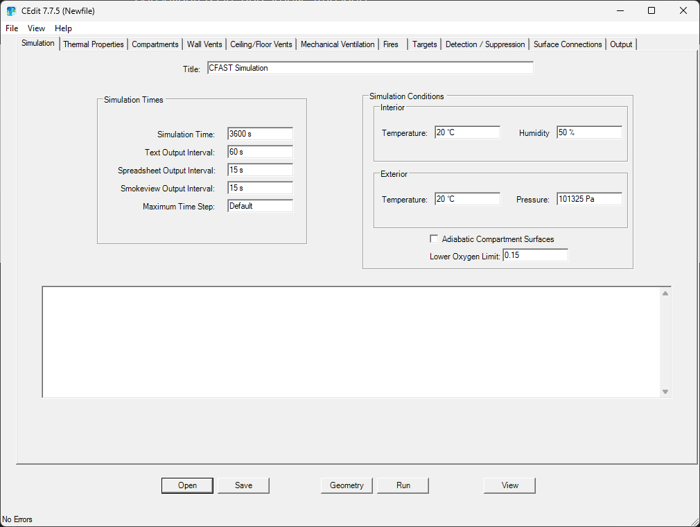
Step 2: Configure Simulation Environment#
The simulation environment defines the global parameters for our CFAST simulation. The
SimulationEnvironment class is the equivalent of the CEdit
simulation settings tab but programmatically defined.
simulation_env = SimulationEnvironment(
    title="Simple example",
    time_simulation=7200,
    print=40,
    smokeview=10,
    spreadsheet=10,
    init_pressure=101325,
    relative_humidity=50,
    interior_temperature=20,
    exterior_temperature=20,
    adiabatic=False,
    lower_oxygen_limit=0.1,
    max_time_step=10,
)
Step 3: Define Material Properties#
Material properties define the thermal characteristics of surfaces in our compartments. The
Material class is the equivalent of the CEdit simulation settings tab but
programmatically defined.
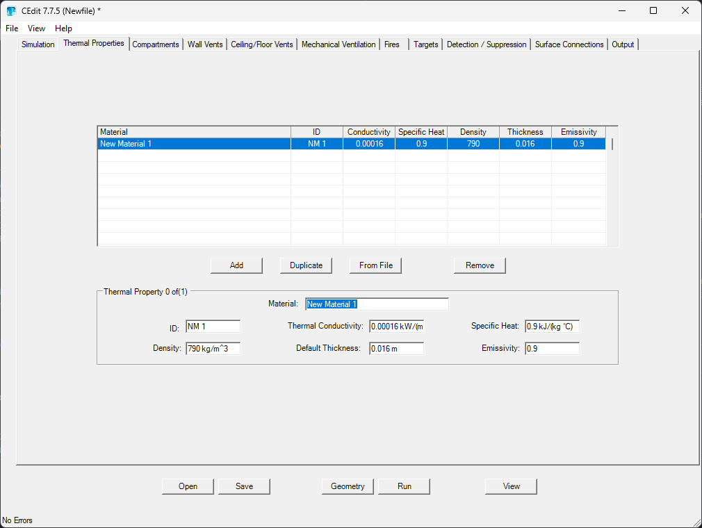
Here we define gypsum board, which is commonly used for walls and ceilings.
gypsum_board = Material(
    id="Gypboard",
    material="Gypsum Board",
    conductivity=0.16,
    density=480,
    specific_heat=1,
    thickness=0.015,
    emissivity=0.9,
)
Step 4: Create Compartment#
Compartment represent the physical spaces in our building. The
Compartment class is the equivalent of the CEdit compartment tab
but programmatically defined.
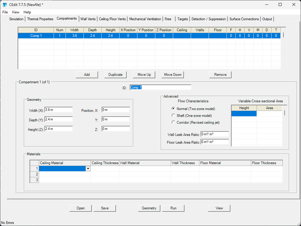
We’ll create two 10×10×10 meter rooms stacked vertically.
ground_level = Compartment(
    id="Comp 1",
    depth=10.0,
    height=10.0,
    width=10.0,
    ceiling_mat_id="Gypboard",
    ceiling_thickness=0.01,
    wall_mat_id="Gypboard",
    wall_thickness=0.01,
    floor_mat_id="Gypboard",
    floor_thickness=0.01,
    origin_x=0,
    origin_y=0,
    origin_z=0,
)

upper_level = Compartment(
    id="Comp 2",
    depth=10.0,
    height=10.0,
    width=10.0,
    ceiling_mat_id="Gypboard",
    ceiling_thickness=0.01,
    wall_mat_id="Gypboard",
    wall_thickness=0.01,
    floor_mat_id="Gypboard",
    floor_thickness=0.01,
    origin_x=0,
    origin_y=0,
    origin_z=10,
)
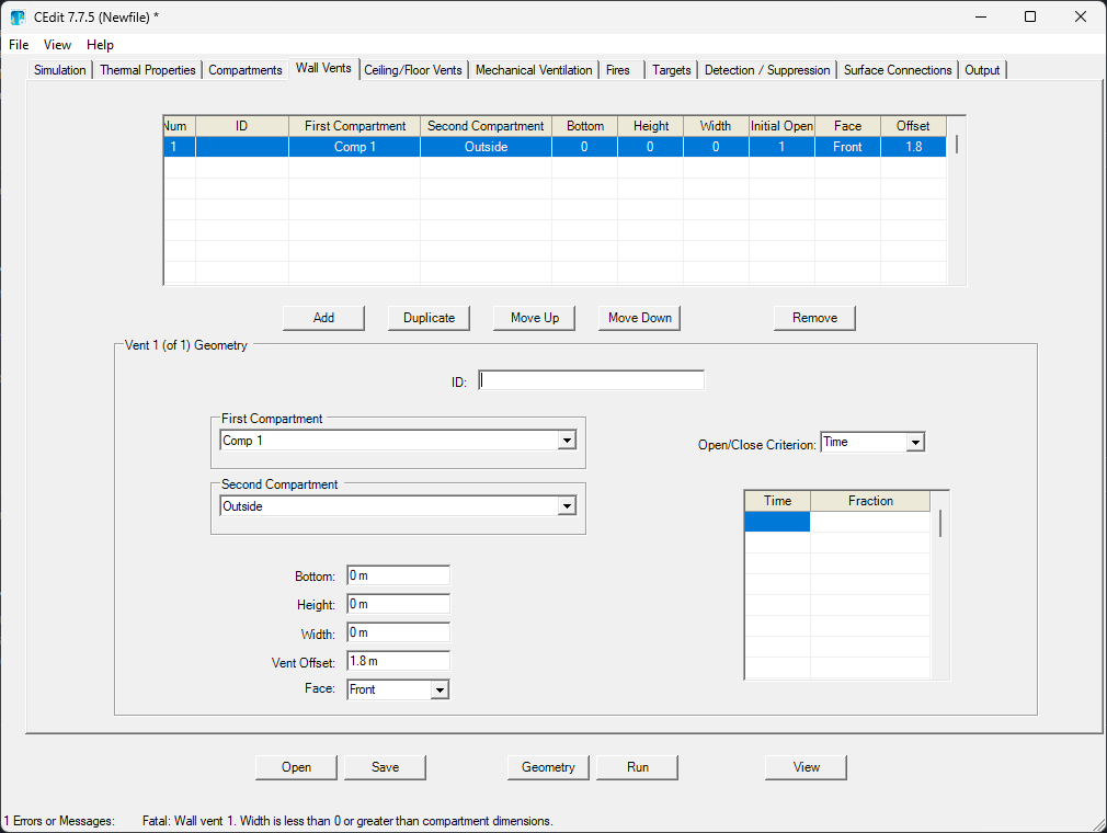
Step 5: Define Ventilation Systems#
As before, we’ll create three types of ventilation:
Wall vents |
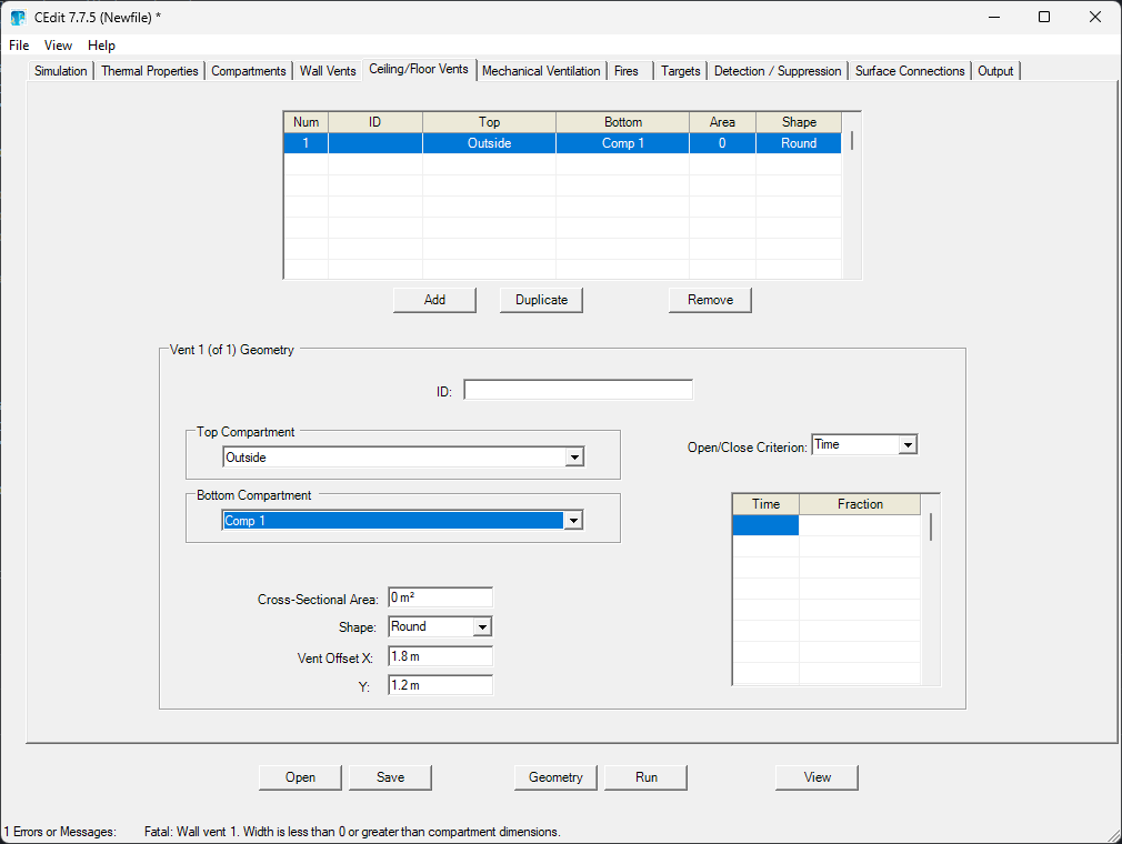
Ceiling/floor vents |
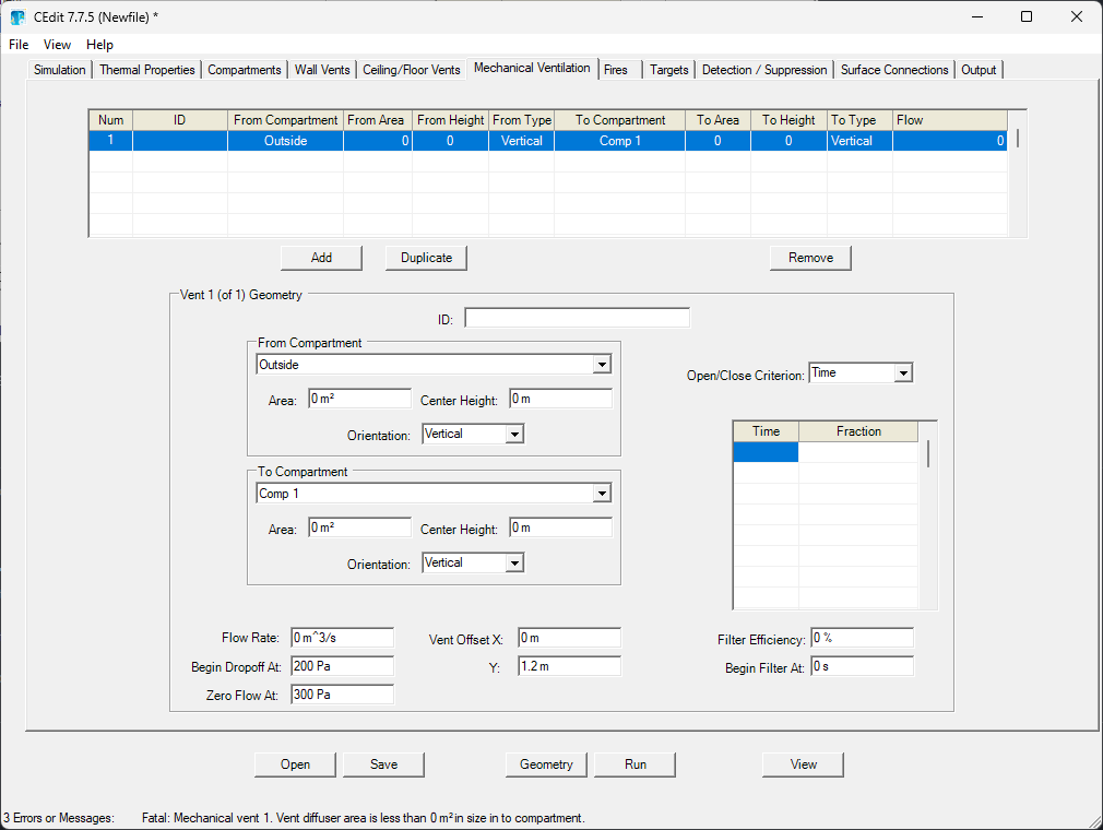
Mechanical vents |
|---|---|---|
Natural ventilation through openings in walls |
Natural ventilation between compartments |
Forced ventilation systems |
|
|
|
We’ll use the MechanicalVent, CeilingFloorVent,
and WallVent classes to define our vents.
# Wall vent connecting first compartment to outside

wall_vent = WallVent(
    id="WallVent_1",
    comps_ids=["Comp 1", "OUTSIDE"],
    bottom=0.02,
    height=0.3,
    width=0.2,
    face="FRONT",
    offset=0.47,
)
ceiling_floor_vents = CeilingFloorVent(
    id="CeilFloorVent_1",
    comps_ids=["Comp 2", "Comp 1"],
    area=0.01,
    shape="SQUARE",
    offsets=[0.84, 0.86],
)

mechanical_vents = MechanicalVent(
    id="mech",
    comps_ids=["OUTSIDE", "Comp 1"],
    area=[1.2, 10],
    heights=[1, 1],
    orientations=["HORIZONTAL", "HORIZONTAL"],
    flow=1,
    cutoffs=[250, 300],
    offsets=[0, 0.6],
    filter_time=1.2,
    filter_efficiency=5,
)
Step 6: Define Fire Sources#
Fire sources represent the combustion processes in our simulation. The
Fire class is the equivalent of the CEdit fires tab
but programmatically defined.
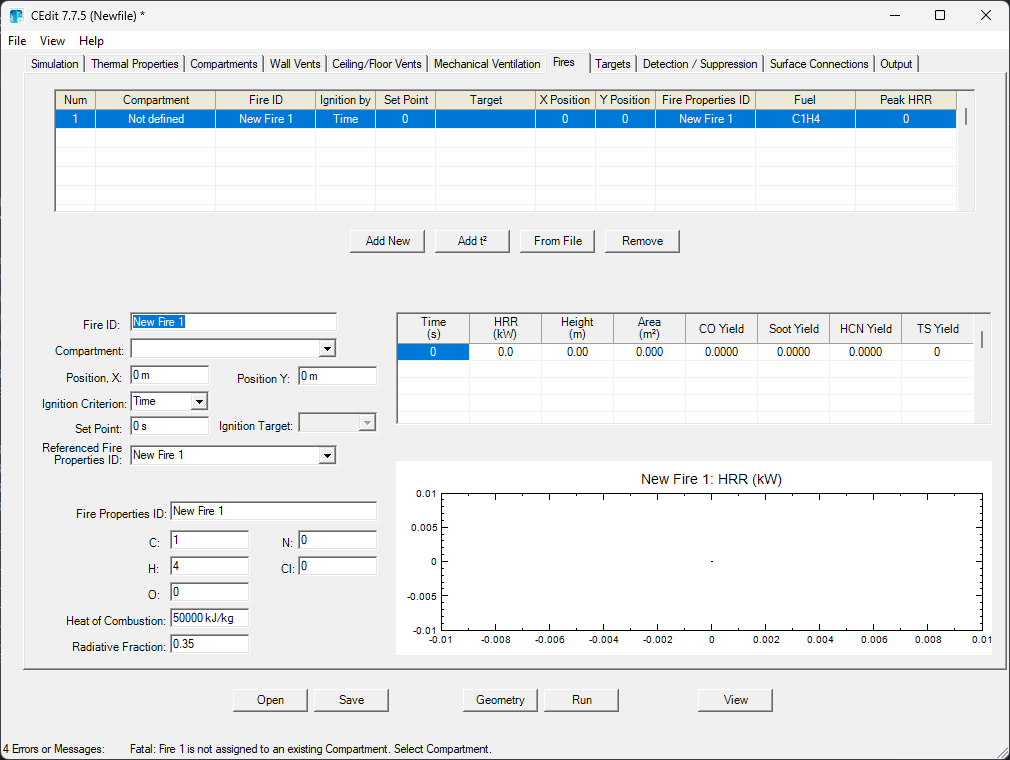
Here we define a propane fire with specific chemical composition and heat release characteristics.
propane_fire = Fire(
    id="Propane",
    comp_id="Comp 1",
    fire_id="Propane_Fire",
    location=[0.3, 0.3],
    carbon=5,
    chlorine=2,
    hydrogen=8,
    nitrogen=1,
    oxygen=0,
    heat_of_combustion=100,
    radiative_fraction=0.3,
    data_table=[
        [0, 0, 0, 0.3, 0.008021683, 0.02, 0, 0, 0],  # t=0s
        [30, 10, 0, 0.3, 0.008021683, 0.02, 0, 0, 0],  # t=30s
        [60, 40, 0, 0.3, 0.008021683, 0.02, 0, 0, 0],  # t=60s
        [90, 90, 0, 0.3, 0.008021683, 0.02, 0, 0, 0],  # t=90s
        [120, 160, 0, 0.3, 0.008021683, 0.02, 0, 0, 0],  # t=120s
        [150, 250, 0, 0.3, 0.008021683, 0.02, 0, 0, 0],  # t=150s
        [180, 360, 0, 0.3, 0.008021683, 0.02, 0, 0, 0],  # t=180s
        [210, 490, 0, 0.3, 0.008021683, 0.02, 0, 0, 0],  # ...
        [240, 640, 0, 0.3, 0.008021683, 0.02, 0, 0, 0],
        [270, 810, 0, 0.3, 0.008021683, 0.02, 0, 0, 0],
        [300, 999.9999, 0, 0.3, 0.008021683, 0.02, 0, 0, 0],
        [600, 1000, 0, 0.3, 0.008021683, 0.02, 0, 0, 0],
        [601, 810, 0, 0.3, 0.008021683, 0.02, 0, 0, 0],
        [602, 640, 0, 0.3, 0.008021683, 0.02, 0, 0, 0],
        [603, 490, 0, 0.3, 0.008021683, 0.02, 0, 0, 0],
        [604, 360, 0, 0.3, 0.008021683, 0.02, 0, 0, 0],
        [605, 250, 0, 0.3, 0.008021683, 0.02, 0, 0, 0],
        [606, 160, 0, 0.3, 0.008021683, 0.02, 0, 0, 0],
        [607, 90, 0, 0.3, 0.008021683, 0.02, 0, 0, 0],
        [608, 40, 0, 0.3, 0.008021683, 0.02, 0, 0, 0],
        [609, 10, 0, 0.3, 0.008021683, 0.02, 0, 0, 0],
        [610, 0, 0, 0.3, 0.008021683, 0.02, 0, 0, 0],
        [620, 0, 0, 0.3, 0.008021683, 0.02, 0, 0, 0],
    ],
)
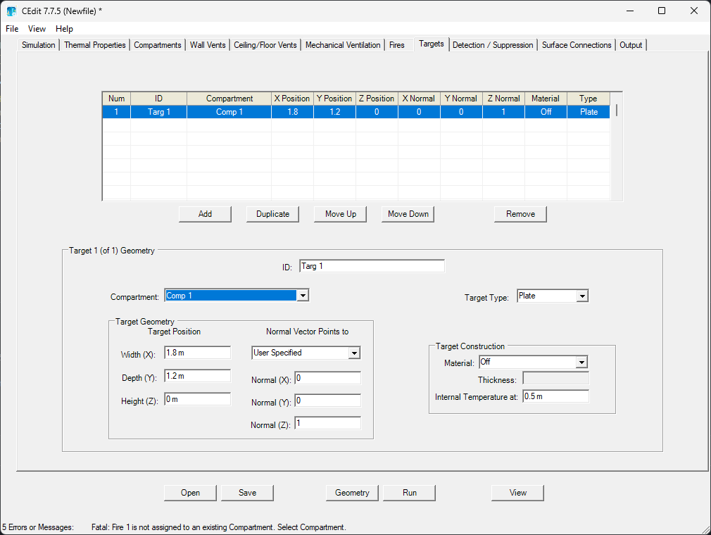
Step 7: Add Device#
Device allow us to monitor conditions at specific locations. The
Device class is the equivalent of the CEdit devices tab but
programmatically defined.
The Device class has classmethods to help create common device types:
create_target: equivalent of target devicecreate_heat_detector: equivalent of heat detector devicecreate_smoke_detector: equivalent of smoke detector devicecreate_sprinkler: equivalent of sprinkler device
Here we add a target device to measure thermal conditions.
target = Device.create_target(
    id="Target_1",
    comp_id="Comp 1",
    location=[0.5, 0.5, 0],
    type="CYLINDER",
    material_id="Gypboard",
    surface_orientation="CEILING",
    thickness=0.01,
    temperature_depth=0.01,
    depth_units="M",
)
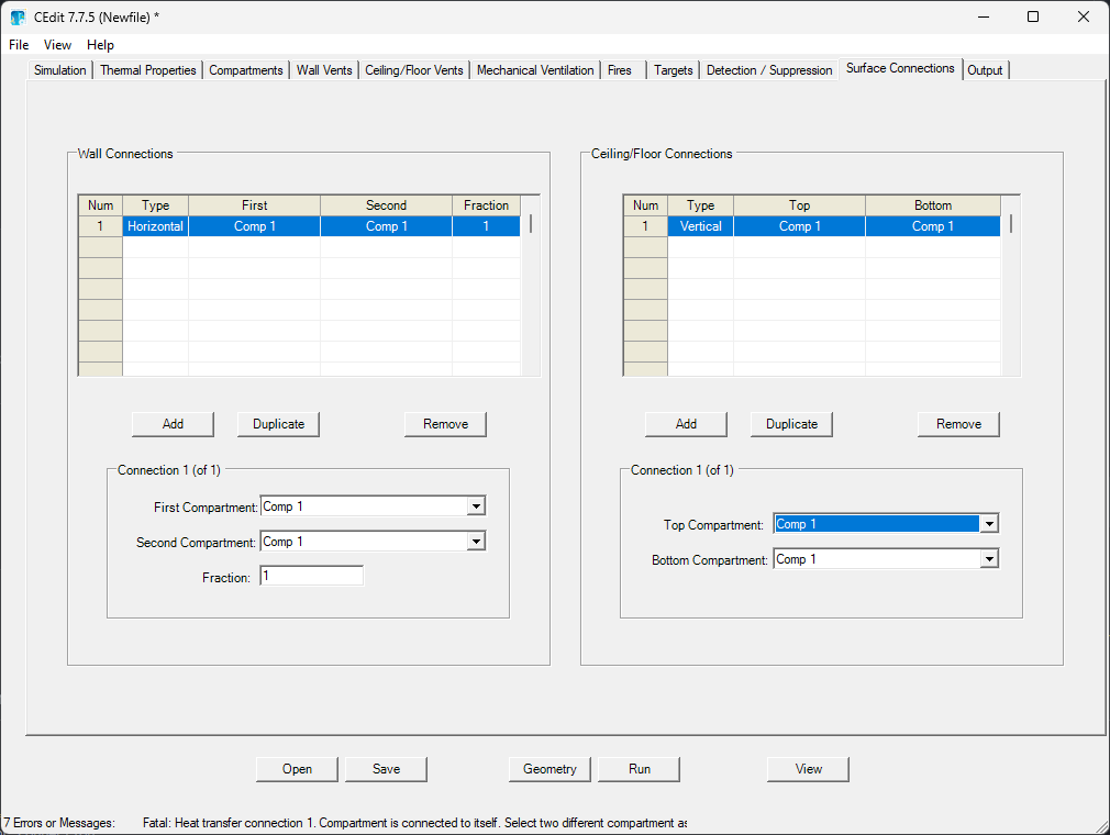
Step 8: Configure Surface Connections#
Surface connections define thermal connections between compartments through shared
surfaces. The SurfaceConnection class is the equivalent of the
CEdit surface connections tab but programmatically defined.
The SurfaceConnection class has 2 classmethods to help create
common connection types ceiling_floor_connection,
and wall_connection. Here we create a
ceiling/floor connection between the two compartments to allow heat transfer and air
flow between them.
ceiling_floor_connection = SurfaceConnection.ceiling_floor_connection(
    comp_id="Comp 1",
    comp_ids="Comp 2",
)
Step 9: Create and Run the CFAST Model#
Now we’ll create a complete CFASTModel with all our components and
run the simulation. After running, we’ll explore how to access and analyze the
results.
model = CFASTModel(
    simulation_environment=simulation_env,
    material_properties=[gypsum_board],
    compartments=[ground_level, upper_level],
    wall_vents=[wall_vent],
    ceiling_floor_vents=[ceiling_floor_vents],
    mechanical_vents=[mechanical_vents],
    fires=[propane_fire],
    devices=[target],
    surface_connections=[ceiling_floor_connection],
    file_name="example_simulation.in",
    cfast_exe="cfast",
    extra_arguments=["-f"],
)
Use the summary method to print a summary of the model
configuration.
print(model.summary())
Model: example_simulation.in
Simulation: 'Simple example' (7200s)

Components:
  Material Properties (1):
    Material 'Gypboard' (Gypsum Board): k=0.16, ρ=480, c=1, t=0.015, ε=0.9
  Compartment (2):
    Compartment 'Comp 1': 10.0x10.0x10.0 m, volume: 1000.00 m³ (ceiling: Gypboard, wall: Gypboard, floor: Gypboard)
    Compartment 'Comp 2': 10.0x10.0x10.0 m, volume: 1000.00 m³ (ceiling: Gypboard, wall: Gypboard, floor: Gypboard)
  Wall Vents (1):
    Wall Vent 'WallVent_1': Comp 1 ↔ OUTSIDE, 0.2x0.3 m, bottom: 0.02 m
  Ceiling/Floor Vents (1):
    Ceiling/Floor Vent 'CeilFloorVent_1': Comp 2 ↕ Comp 1, area: 0.01 m², shape: SQUARE
  Mechanical Vents (1):
    Mechanical Vent 'mech': OUTSIDE -> Comp 1, flow: 1 m³/s
  Fire (1):
    Fire 'Propane' (Propane_Fire) in 'Comp 1' at (0.3, 0.3) (peak: 1 kW, duration: 10min, χr: 0.3)
  Device (1):
    Target 'Target_1' (CYLINDER) in 'Comp 1' at (0.5, 0.5, 0) (material: Gypboard, depth: 0.01m, thickness: 0.01m)
  Surface Connections (1):
    Surface Connection (FLOOR): Comp 1 -> Comp 2
You can also save to the disk the CFAST model input file with the
save method and view its contents with
view_cfast_input_file (not necessary to run the
simulation, as the model will be saved automatically when you run it, but useful if
you want to inspect the generated input file or run it manually with CFAST).
model.save()

input_file_contents = model.view_cfast_input_file(pretty_print=True)
print(input_file_contents)
 1: &HEAD VERSION = 7700 TITLE = 'Simple example' /
 2:
 3: !! Scenario Configuration
 4: &TIME SIMULATION = 7200 PRINT = 40 SMOKEVIEW = 10 SPREADSHEET = 10 /
 5: &INIT PRESSURE = 101325 RELATIVE_HUMIDITY = 50 INTERIOR_TEMPERATURE = 20 EXTERIOR_TEMPERATURE = 20 /
 6: &MISC ADIABATIC = .FALSE. MAX_TIME_STEP = 10 LOWER_OXYGEN_LIMIT = 0.1 /
 7:
 8: !! Material Properties
 9: &MATL ID = 'Gypboard' MATERIAL = 'Gypsum Board' CONDUCTIVITY = 0.16 DENSITY = 480 SPECIFIC_HEAT = 1 THICKNESS = 0.015 EMISSIVITY = 0.9 /
10:
11: !! Compartments
12: &COMP ID = 'Comp 1' DEPTH = 10.0 HEIGHT = 10.0 WIDTH = 10.0 CEILING_MATL_ID = 'Gypboard' CEILING_THICKNESS = 0.01 WALL_MATL_ID = 'Gypboard' WALL_THICKNESS = 0.01 FLOOR_MATL_ID = 'Gypboard' FLOOR_THICKNESS = 0.01 ORIGIN = 0, 0, 0 GRID = 50, 50, 50 /
13: &COMP ID = 'Comp 2' DEPTH = 10.0 HEIGHT = 10.0 WIDTH = 10.0 CEILING_MATL_ID = 'Gypboard' CEILING_THICKNESS = 0.01 WALL_MATL_ID = 'Gypboard' WALL_THICKNESS = 0.01 FLOOR_MATL_ID = 'Gypboard' FLOOR_THICKNESS = 0.01 ORIGIN = 0, 0, 10 GRID = 50, 50, 50 /
14:
15: !! Wall Vents
16: &VENT TYPE = 'WALL' ID = 'WallVent_1' COMP_IDS = 'Comp 1', 'OUTSIDE' BOTTOM = 0.02 HEIGHT = 0.3 WIDTH = 0.2 FACE = 'FRONT' OFFSET = 0.47 /
17:
18: !! Ceiling and Floor Vents
19: &VENT TYPE = 'FLOOR' ID = 'CeilFloorVent_1' COMP_IDS = 'Comp 2', 'Comp 1' AREA = 0.01 SHAPE = 'SQUARE' OFFSETS = 0.84, 0.86 /
20:
21: !! Mechanical Vents
22: &VENT TYPE = 'MECHANICAL' ID = 'mech' COMP_IDS = 'OUTSIDE', 'Comp 1' AREAS = 1.2, 10 HEIGHTS = 1, 1 ORIENTATIONS = 'HORIZONTAL', 'HORIZONTAL' FLOW = 1 CUTOFFS = 250, 300 OFFSETS = 0, 0.6 FILTER_TIME = 1.2 FILTER_EFFICIENCY = 5 /
23:
24: !! Fire
25: &FIRE ID = 'Propane' COMP_ID = 'Comp 1' FIRE_ID = 'Propane_Fire' LOCATION = 0.3, 0.3 /
26: &CHEM ID = 'Propane_Fire' CARBON = 5 CHLORINE = 2 HYDROGEN = 8 NITROGEN = 1 OXYGEN = 0 HEAT_OF_COMBUSTION = 100 RADIATIVE_FRACTION = 0.3 /
27: &TABL ID = 'Propane_Fire' LABELS = 'TIME', 'HRR', 'HEIGHT', 'AREA', 'CO_YIELD', 'SOOT_YIELD', 'HCN_YIELD', 'HCL_YIELD', 'TRACE_YIELD' /
28: &TABL ID = 'Propane_Fire' DATA = 0.0, 0.0, 0.0, 0.3, 0.008021683, 0.02, 0.0, 0.0, 0.0 /
29: &TABL ID = 'Propane_Fire' DATA = 30.0, 10.0, 0.0, 0.3, 0.008021683, 0.02, 0.0, 0.0, 0.0 /
30: &TABL ID = 'Propane_Fire' DATA = 60.0, 40.0, 0.0, 0.3, 0.008021683, 0.02, 0.0, 0.0, 0.0 /
31: &TABL ID = 'Propane_Fire' DATA = 90.0, 90.0, 0.0, 0.3, 0.008021683, 0.02, 0.0, 0.0, 0.0 /
32: &TABL ID = 'Propane_Fire' DATA = 120.0, 160.0, 0.0, 0.3, 0.008021683, 0.02, 0.0, 0.0, 0.0 /
33: &TABL ID = 'Propane_Fire' DATA = 150.0, 250.0, 0.0, 0.3, 0.008021683, 0.02, 0.0, 0.0, 0.0 /
34: &TABL ID = 'Propane_Fire' DATA = 180.0, 360.0, 0.0, 0.3, 0.008021683, 0.02, 0.0, 0.0, 0.0 /
35: &TABL ID = 'Propane_Fire' DATA = 210.0, 490.0, 0.0, 0.3, 0.008021683, 0.02, 0.0, 0.0, 0.0 /
36: &TABL ID = 'Propane_Fire' DATA = 240.0, 640.0, 0.0, 0.3, 0.008021683, 0.02, 0.0, 0.0, 0.0 /
37: &TABL ID = 'Propane_Fire' DATA = 270.0, 810.0, 0.0, 0.3, 0.008021683, 0.02, 0.0, 0.0, 0.0 /
38: &TABL ID = 'Propane_Fire' DATA = 300.0, 999.9999, 0.0, 0.3, 0.008021683, 0.02, 0.0, 0.0, 0.0 /
39: &TABL ID = 'Propane_Fire' DATA = 600.0, 1000.0, 0.0, 0.3, 0.008021683, 0.02, 0.0, 0.0, 0.0 /
40: &TABL ID = 'Propane_Fire' DATA = 601.0, 810.0, 0.0, 0.3, 0.008021683, 0.02, 0.0, 0.0, 0.0 /
41: &TABL ID = 'Propane_Fire' DATA = 602.0, 640.0, 0.0, 0.3, 0.008021683, 0.02, 0.0, 0.0, 0.0 /
42: &TABL ID = 'Propane_Fire' DATA = 603.0, 490.0, 0.0, 0.3, 0.008021683, 0.02, 0.0, 0.0, 0.0 /
43: &TABL ID = 'Propane_Fire' DATA = 604.0, 360.0, 0.0, 0.3, 0.008021683, 0.02, 0.0, 0.0, 0.0 /
44: &TABL ID = 'Propane_Fire' DATA = 605.0, 250.0, 0.0, 0.3, 0.008021683, 0.02, 0.0, 0.0, 0.0 /
45: &TABL ID = 'Propane_Fire' DATA = 606.0, 160.0, 0.0, 0.3, 0.008021683, 0.02, 0.0, 0.0, 0.0 /
46: &TABL ID = 'Propane_Fire' DATA = 607.0, 90.0, 0.0, 0.3, 0.008021683, 0.02, 0.0, 0.0, 0.0 /
47: &TABL ID = 'Propane_Fire' DATA = 608.0, 40.0, 0.0, 0.3, 0.008021683, 0.02, 0.0, 0.0, 0.0 /
48: &TABL ID = 'Propane_Fire' DATA = 609.0, 10.0, 0.0, 0.3, 0.008021683, 0.02, 0.0, 0.0, 0.0 /
49: &TABL ID = 'Propane_Fire' DATA = 610.0, 0.0, 0.0, 0.3, 0.008021683, 0.02, 0.0, 0.0, 0.0 /
50: &TABL ID = 'Propane_Fire' DATA = 620.0, 0.0, 0.0, 0.3, 0.008021683, 0.02, 0.0, 0.0, 0.0 /
51:
52: !! Device
53: &DEVC ID = 'Target_1' COMP_ID = 'Comp 1' LOCATION = 0.5, 0.5, 0 TYPE = 'CYLINDER' MATL_ID = 'Gypboard' SURFACE_ORIENTATION = 'CEILING' THICKNESS = 0.01 TEMPERATURE_DEPTH = 0.01 DEPTH_UNITS = 'M' /
54:
55: !! Surface Connections
56: &CONN TYPE = 'FLOOR' COMP_ID = 'Comp 1' COMP_IDS = 'Comp 2' /
57:
58: &TAIL /
The run method returns a dictionary containing
DataFrame for each CFAST output file. This makes it easy to analyze
and visualize the simulation results using familiar pandas methods and matplotlib.
results = model.run(
    verbose=True,
    timeout=None,
)
Available Output Files#
Each simulation generates several CSV files with different types of data:
Key |
Description |
|---|---|
|
Complete zone data including temperatures, pressures, and fire parameters |
|
Target device responses (temperatures, heat fluxes) |
|
Ventilation mass flows through each vent |
|
Detailed compartment conditions for all species |
|
Wall surface temperatures |
|
Species mass tracking over time |
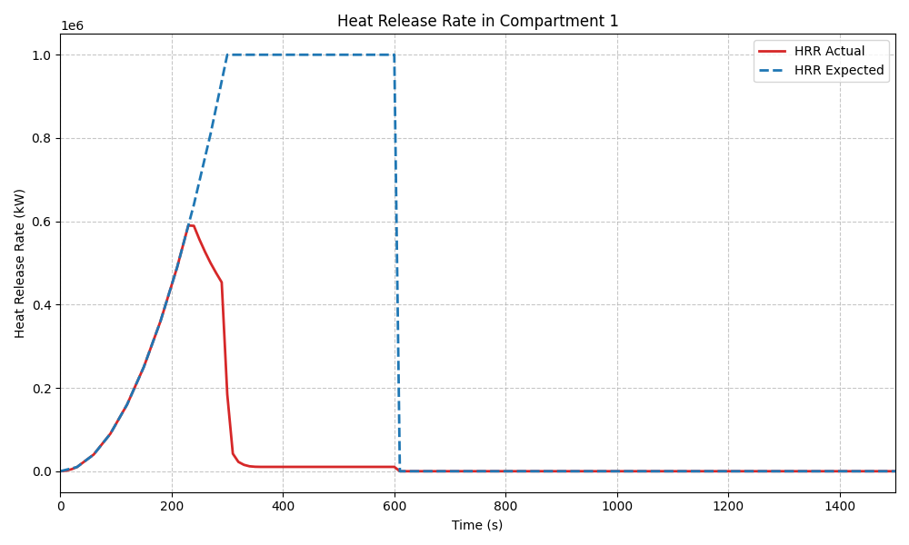
Step 10: Analyzing Simulation Results#
Below is a small example of comparing the Expected HRR and the Actual HRR using matplotlib and pandas, though you’re free to use any Python data analysis tools in the ecosystem!
import matplotlib.pyplot as plt

df = results["compartments"]

plt.figure(figsize=(10, 6))
plt.plot(df["Time"], df["HRR_1"], label="HRR Actual", color="tab:red", linewidth=2)
plt.plot(
    df["Time"],
    df["HRR_E1"],
    label="HRR Expected",
    color="tab:blue",
    linestyle="--",
    linewidth=2,
)
plt.title("Heat Release Rate in Compartment 1")
plt.xlabel("Time (s)")
plt.ylabel("Heat Release Rate (kW)")
plt.legend()
plt.xlim(0, 1500)
plt.grid(True, linestyle="--", alpha=0.7)
plt.tight_layout()
plt.show()
Step 11: Updating the model#
You can update any part of the model after its creation with the update_* methods
(e.g., update_fire_params). For example, to change the
fire’s radiative fraction, you can do:
Original model
[Fire(id='Propane', comp_id='Comp 1', fire_id='Propane_Fire', location=[0.3, 0.3], heat_of_combustion=100, radiative_fraction=0.3, data_rows=23)]
Updated model
new_model = model.update_fire_params(fire="Propane", radiative_fraction=0.4)
new_model.fires
[Fire(id='Propane', comp_id='Comp 1', fire_id='Propane_Fire', location=[0.3, 0.3], heat_of_combustion=100, radiative_fraction=0.4, data_rows=23)]
You can also add additional components to an existing model with
add. For example, to add another
target device:
Original model devices
for device in model.devices:
    print(device)
Target 'Target_1' (CYLINDER) in 'Comp 1' at (0.5, 0.5, 0) (material: Gypboard, depth: 0.01m, thickness: 0.01m)
Adding a new device
new_device = Device.create_target(
    id="Target_2",
    comp_id="Comp 2",
    location=[0.5, 0.5, 0.5],
    type="CYLINDER",
    material_id="Gypboard",
    surface_orientation="CEILING",
    thickness=0.01,
    temperature_depth=0.01,
    depth_units="M",
)

updated_model = model.add(new_device)
And now the updated model has both devices
for device in updated_model.devices:
    print(device)
Target 'Target_1' (CYLINDER) in 'Comp 1' at (0.5, 0.5, 0) (material: Gypboard, depth: 0.01m, thickness: 0.01m)
Target 'Target_2' (CYLINDER) in 'Comp 2' at (0.5, 0.5, 0.5) (material: Gypboard, depth: 0.01m, thickness: 0.01m)
Cleanup#
Finally, we clean up the temporary files generated during the simulation.
import glob
import os

files_to_remove = glob.glob("example_simulation*")

for file in files_to_remove:
    if os.path.exists(file):
        os.remove(file)
        print(f"Removed {file}")

if files_to_remove:
    print("Cleanup completed!")
else:
    print("No files to clean up.")
Removed example_simulation.smv
Removed example_simulation.status
Removed example_simulation_vents.csv
Removed example_simulation_compartments.csv
Removed example_simulation.plt
Removed example_simulation_devices.csv
Removed example_simulation.in
Removed example_simulation.out
Removed example_simulation.log
Removed example_simulation_zone.csv
Removed example_simulation_masses.csv
Removed example_simulation_walls.csv
Cleanup completed!
Total running time of the script: (0 minutes 1.153 seconds)