Note
Go to the end to download the full example code.
04 Sensitivity Analysis#
This example demonstrates how to perform sensitivity analysis on CFAST fire simulation models using the SALib library. We’ll use Sobol indices to quantify parameter importance and visualize the results.
Step 1: Import Required Libraries#
We’ll import:
NumPy: For generating parameter ranges and arrays
Pandas: For organizing and analyzing simulation results
Matplotlib: For visualizing the generated data
SALib: For performing sensitivity analysis (see
sampleandanalyze)PyCFAST: For parsing and running CFAST models (see
parse_cfast_fileandrun)
import matplotlib.pyplot as plt
import numpy as np
import pandas as pd
from matplotlib.ticker import FormatStrFormatter
from SALib.analyze import sobol as sobol_analyze
from SALib.sample import sobol as sobol_sample

from pycfast.parsers import parse_cfast_file
Step 2: Load Base Model#
For this example, we’ll use a predefined CFAST input file as our base model.
You can replace this with your own model file. We’ll use
parse_cfast_file to load the
USN_Hawaii_Test_03.in input file.
model = parse_cfast_file("data/USN_Hawaii_Test_03.in")
The parsed model is displayed below.
print(model.summary())
Model: USN_Hawaii_Test_03_parsed.in
Simulation: 'HawaiiTest 3' (570s)

Components:
  Material Properties (2):
    Material 'CONCRETE' (Concrete Normal Weight (6 in)): k=1.6, ρ=2400.0, c=0.75, t=0.15, ε=0.94
    Material 'STEELSHT' (Steel Plain Carbon (1/16 in)): k=60.0, ρ=7850.0, c=0.48, t=0.0015, ε=0.9
  Compartment (1):
    Compartment 'Bay 1': 97.6x74.0x14.8 m, volume: 106891.52 m³ (ceiling: CONCRETE, wall: CONCRETE, floor: CONCRETE)
  Fire (1):
    Fire 'Hawaii_03' (Hawaii_03_Fire) in 'Bay 1' at (36.7, 39.9) (peak: 1 kW, duration: 11min, χr: 0.4)
  Device (1):
    Target 'Targ 1' (PLATE) in 'Bay 1' at (36.7, 39.9, 14.7) (material: STEELSHT, depth: 0.00075m)
Step 3: Define the Problem for Sensitivity Analysis#
We specify which parameters to analyze and their realistic ranges. For this example, we focus on four key parameters:
Heat of combustion: Energy released per unit mass of fuel (affects fire intensity)
Radiative fraction: Fraction of fire energy released as radiation (affects heat transfer)
Target thickness: Material thickness of temperature measurement targets
Target emissivity: Surface radiation properties of targets
Each parameter gets a range of realistic values to explore during the analysis.
problem = {
    "num_vars": 4,
    "names": [
        "heat_of_combustion",
        "radiative_fraction",
        "target_thickness",
        "target_emissivity",
    ],
    "bounds": [
        [100, 50000],
        [0.1, 0.8],
        [0.10, 0.60],
        [0.8, 0.95],
    ],
}
Below you can see the defined parameters and their ranges for the sensitivity analysis.
heat_of_combustion: [100, 50000]
radiative_fraction: [0.1, 0.8]
target_thickness: [0.1, 0.6]
target_emissivity: [0.8, 0.95]
Step 4: Generate Parameter Samples#
We use Sobol sequences to create well-distributed parameter combinations. The number of samples affects accuracy but also computational time.
N = 64  # Number of samples (will generate N*(2*num_vars+2) total samples)
param_values = sobol_sample.sample(problem, N)

print(f"Generated {len(param_values)} parameter combinations")
print(f"Sample shape: {param_values.shape}")

df_samples = pd.DataFrame(param_values, columns=problem["names"])
Generated 640 parameter combinations
Sample shape: (640, 4)
First 5 parameter combinations
Step 5: Run Model Evaluations#
Now we run CFAST simulations for each parameter combination. This is the most time-consuming step as we need to:
Modify the model with each parameter set using
update_fire_paramsandupdate_material_paramsRun the CFAST simulation with
runExtract and store the output values
outputs = []

for i, params in enumerate(param_values):
    if i % 50 == 0:
        print(
            f"Sample {i}/{len(param_values)}: "
            f"hoc={params[0]}, rf={params[1]}, thickness={params[2]}, emissivity={params[3]}"
        )

    temp_model = model.update_fire_params(
        fire="Hawaii_03_Fire",
        heat_of_combustion=params[0],
        radiative_fraction=params[1],
    )
    temp_model = temp_model.update_material_params(
        material="STEELSHT",
        thickness=params[2],
        emissivity=params[3],
    )

    results = temp_model.run()
    max_target_temp = results["devices"]["TRGSURT_1"].max()

    outputs.append(max_target_temp)

Y = np.array(outputs)
print(f"Completed {len(outputs)} model evaluations")
print(f"Output shape: {Y.shape}")
Sample 0/640: hoc=512.0456199161708, rf=0.41330568864941597, thickness=0.4315482260659337, emissivity=0.9289455804042518
Sample 50/640: hoc=37519.90600191057, rf=0.7574261432513595, thickness=0.40060999607667325, emissivity=0.9094802263192833
Sample 100/640: hoc=31422.973106708378, rf=0.37806312805041675, thickness=0.12055288292467595, emissivity=0.9315452500246465
Sample 150/640: hoc=5817.869811505079, rf=0.732448357809335, thickness=0.21459987098351122, emissivity=0.8786837472580373
Sample 200/640: hoc=21711.08831530437, rf=0.4053006402216852, thickness=0.3211018851958215, emissivity=0.888432411942631
Sample 250/640: hoc=48998.45961648971, rf=0.5363889450207353, thickness=0.42138042617589233, emissivity=0.8838962375652045
Sample 300/640: hoc=39950.94994781539, rf=0.42952006384730346, thickness=0.5110192083753645, emissivity=0.8998963889665902
Sample 350/640: hoc=13315.61574647203, rf=0.6116318213753402, thickness=0.500614196434617, emissivity=0.8850074601359665
Sample 400/640: hoc=6692.366825137287, rf=0.3704486040398479, thickness=0.55807491755113, emissivity=0.8505420302506537
Sample 450/640: hoc=30549.285280890763, rf=0.7126991033554078, thickness=0.5270169259980321, emissivity=0.8284446959849447
Sample 500/640: hoc=28737.697797082365, rf=0.20071716327220201, thickness=0.17373441196978093, emissivity=0.9108160256408154
Sample 550/640: hoc=9273.029607255012, rf=0.5544177118688822, thickness=0.1427988045848906, emissivity=0.9288554101251065
Sample 600/640: hoc=15122.599057573825, rf=0.4496117827482522, thickness=0.1986041994765401, emissivity=0.8168451014440508
Completed 640 model evaluations
Output shape: (640,)
Step 6: Perform Sobol Sensitivity Analysis#
We calculate Sobol indices to quantify parameter importance:
First-order indices (S1): Direct effect of each parameter alone
Total-order indices (ST): Total effect including interactions with other parameters
Interaction effects (ST - S1): How much parameters interact with each other
Higher values indicate greater influence on the simulation output.
First-order indices (S1):
for i, param_name in enumerate(problem["names"]):
    print(f"{param_name}: {Si['S1'][i]:.4f}")
heat_of_combustion: 0.4726
radiative_fraction: 0.2406
target_thickness: 0.1796
target_emissivity: 0.0251
Total-order indices (ST):
for i, param_name in enumerate(problem["names"]):
    print(f"{param_name}: {Si['ST'][i]:.4f}")
heat_of_combustion: 0.5571
radiative_fraction: 0.3906
target_thickness: 0.1794
target_emissivity: 0.0295
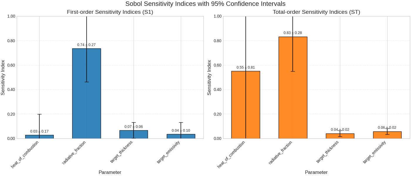
Step 7: Visualize Sensitivity Results#
The bar charts show:
Left panel: First-order effects (direct parameter influence)
Right panel: Total effects (including parameter interactions)
Error bars: Confidence intervals for the estimates
Parameters with higher bars have greater influence on the simulation output. Large differences between S1 and ST indicate significant parameter interactions.
plt.style.use("seaborn-v0_8-whitegrid")

fig, (ax1, ax2) = plt.subplots(1, 2, figsize=(14, 6), constrained_layout=True)

names = problem["names"]
x = np.arange(len(names))

S1 = np.asarray(Si["S1"])
S1_conf = np.asarray(Si["S1_conf"])
ST = np.asarray(Si["ST"])
ST_conf = np.asarray(Si["ST_conf"])

cmap = plt.get_cmap("tab10")
bar_width = 0.6

ymax_candidate = np.nanmax([S1 + S1_conf, ST + ST_conf])
ymax = (
    float(np.clip(ymax_candidate + 0.06, 0, 1.0))
    if not np.isnan(ymax_candidate)
    else 1.0
)
ymin = 0.0

ax1.bar(x, S1, width=bar_width, color=cmap(0), edgecolor="black", alpha=0.9)
ax1.errorbar(
    x, S1, yerr=S1_conf, fmt="none", ecolor="black", capsize=5, elinewidth=1.25
)
ax1.set_title("First-order Sensitivity Indices (S1)", fontsize=14)
ax1.set_ylabel("Sensitivity Index", fontsize=12)
ax1.set_xlabel("Parameter", fontsize=12)
ax1.set_xticks(x)
ax1.set_xticklabels(names, rotation=45, ha="right", fontsize=10)
ax1.set_ylim(ymin, ymax)
ax1.grid(which="major", axis="y", linestyle="--", alpha=0.4)

for i, v in enumerate(S1):
    if np.isnan(v):
        txt = "nan"
    else:
        txt = f"{v:.2f} ± {S1_conf[i]:.2f}"
    ax1.text(
        i,
        (v if not np.isnan(v) else 0) + (0.02 if not np.isnan(v) else 0.01),
        txt,
        ha="center",
        fontsize=9,
    )

ax2.bar(x, ST, width=bar_width, color=cmap(1), edgecolor="black", alpha=0.9)
ax2.errorbar(
    x, ST, yerr=ST_conf, fmt="none", ecolor="black", capsize=5, elinewidth=1.25
)
ax2.set_title("Total-order Sensitivity Indices (ST)", fontsize=14)
ax2.set_ylabel("Sensitivity Index", fontsize=12)
ax2.set_xlabel("Parameter", fontsize=12)
ax2.set_xticks(x)
ax2.set_xticklabels(names, rotation=45, ha="right", fontsize=10)
ax2.set_ylim(ymin, ymax)
ax2.grid(which="major", axis="y", linestyle="--", alpha=0.4)

for i, v in enumerate(ST):
    if np.isnan(v):
        txt = "nan"
    else:
        txt = f"{v:.2f} ± {ST_conf[i]:.2f}"
    ax2.text(
        i,
        (v if not np.isnan(v) else 0) + (0.02 if not np.isnan(v) else 0.01),
        txt,
        ha="center",
        fontsize=9,
    )

ax1.yaxis.set_major_formatter(FormatStrFormatter("%.2f"))
ax2.yaxis.set_major_formatter(FormatStrFormatter("%.2f"))

for ax in (ax1, ax2):
    ax.axhline(0, color="gray", linewidth=0.8)
    ax.set_ylim(bottom=ymin)

plt.suptitle("Sobol Sensitivity Indices with 95% Confidence Intervals", fontsize=16)
plt.show()

interaction_effects = ST - S1
print("Interaction Effects (ST - S1):")
for i, param_name in enumerate(names):
    val = interaction_effects[i]
    if np.isnan(val):
        print(f"{param_name}: nan")
    else:
        tag = "(interactions dominant)" if val > 0.05 else ""
        print(f"{param_name}: {val:.3f}{tag}")
Interaction Effects (ST - S1):
heat_of_combustion: 0.084(interactions dominant)
radiative_fraction: 0.150(interactions dominant)
target_thickness: -0.000
target_emissivity: 0.004
Cleanup#
CFAST generates temporary output files during simulation runs. We clean these up to keep the workspace tidy and avoid confusion with future runs.
import glob
import os

files_to_remove = glob.glob("USN_Hawaii_Test_03*")

for file in files_to_remove:
    if os.path.exists(file):
        os.remove(file)
        print(f"Removed {file}")

if files_to_remove:
    print("Cleanup completed!")
else:
    print("No files to clean up.")
Removed USN_Hawaii_Test_03_parsed.smv
Removed USN_Hawaii_Test_03_parsed_walls.csv
Removed USN_Hawaii_Test_03_parsed.status
Removed USN_Hawaii_Test_03_parsed.in
Removed USN_Hawaii_Test_03_parsed.plt
Removed USN_Hawaii_Test_03_parsed.log
Removed USN_Hawaii_Test_03_parsed_zone.csv
Removed USN_Hawaii_Test_03_parsed_vents.csv
Removed USN_Hawaii_Test_03_parsed_compartments.csv
Removed USN_Hawaii_Test_03_parsed.out
Removed USN_Hawaii_Test_03_parsed_devices.csv
Removed USN_Hawaii_Test_03_parsed_masses.csv
Cleanup completed!
Total running time of the script: (1 minutes 31.608 seconds)