03 Generating Data with PyCFAST

This example demonstrates how to use PyCFAST with NumPy to generate simulation data by running multiple CFAST fire simulations with varying parameters.

We’ll create a simple parametric study by varying fire characteristics and analyze the trends in the results.

Step 1: Import Libraries

We’ll import:

• NumPy: For generating parameter ranges and arrays

• Pandas: For organizing and analyzing simulation results

• Matplotlib: For visualizing the generated data

• PyCFAST: For parsing and running CFAST models (see parse_cfast_file() and run())

import os

import matplotlib.pyplot as plt
import numpy as np

from pycfast.parsers import parse_cfast_file

Step 2: Load Base Model

We start with an existing CFAST model as our template. We’ll use USN_Hawaii_Test_03.in. This model serves as the foundation that we’ll modify systematically to generate our dataset.

model = parse_cfast_file("data/USN_Hawaii_Test_03.in")

The parsed model is displayed below.

model

🔥

CFAST Model

USN_Hawaii_Test_03_parsed.in

Total Components: 5

Simulation: HawaiiTest 3

Duration: 10 min

Compartments (1)

• Bay 1: 97.6×74.0×14.8 m

Fires (1)

• Hawaii_03 in Bay 1: Hawaii_03_Fire

Devices (1)

• Targ 1 in Bay 1: PLATE

Materials (2)

• CONCRETE: Concrete Normal Weight (6 in)
• STEELSHT: Steel Plain Carbon (1/16 in)

Step 3: Generate Parameter Combinations

We use NumPy to create systematic parameter variations. For this study, we’ll vary two key fire parameters:

• Heat of combustion: Energy released per unit mass of fuel (affects fire intensity)

• Radiative fraction: Portion of fire energy released as radiation (affects heat transfer)

n_samples = 10

heat_of_combustion_values = np.linspace(15, 5000, n_samples)  # MJ/kg
radiative_fraction_values = np.linspace(0.1, 0.9, n_samples)  # Fraction

parameter_combinations = list(
    zip(heat_of_combustion_values, radiative_fraction_values, strict=False)
)

print(f"Generated {len(parameter_combinations)} parameter combinations")
print(
    f"Heat of combustion range: {heat_of_combustion_values[0]:.2f} - {heat_of_combustion_values[-1]:.2f} MJ/kg"
)
print(
    f"Radiative fraction range: {radiative_fraction_values[0]:.2f} - {radiative_fraction_values[-1]:.2f}"
)

Generated 10 parameter combinations
Heat of combustion range: 15.00 - 5000.00 MJ/kg
Radiative fraction range: 0.10 - 0.90

Step 4: Run Parametric Study

Now we’ll systematically modify the model parameters and run simulations to generate our dataset.

This creates a structured dataset linking input parameters to simulation outputs.

all_runs = []

for i, (hoc, rf) in enumerate(parameter_combinations):
    print(
        f"Running simulation {i + 1}/{len(parameter_combinations)}: hoc={hoc}, rf={rf}"
    )

    # Update fire parameters using :meth:`~pycfast.CFASTModel.update_fire_params`
    temp_model = model.update_fire_params(
        fire="Hawaii_03_Fire", heat_of_combustion=hoc, radiative_fraction=rf
    )

    # Run the simulation with :meth:`~pycfast.CFASTModel.run` and save the output
    outputs = temp_model.run(file_name=f"data_gen_sim_{i:03d}.in")
    all_runs.append(
        {
            "simulation_id": i,
            "hoc": hoc,  # heat of combustion
            "rf": rf,  # radiative fraction
            "outputs": outputs,
        }
    )

Running simulation 1/10: hoc=15.0, rf=0.1
Running simulation 2/10: hoc=568.8888888888889, rf=0.18888888888888888
Running simulation 3/10: hoc=1122.7777777777778, rf=0.2777777777777778
Running simulation 4/10: hoc=1676.6666666666667, rf=0.3666666666666667
Running simulation 5/10: hoc=2230.5555555555557, rf=0.4555555555555556
Running simulation 6/10: hoc=2784.4444444444443, rf=0.5444444444444445
Running simulation 7/10: hoc=3338.3333333333335, rf=0.6333333333333333
Running simulation 8/10: hoc=3892.2222222222226, rf=0.7222222222222222
Running simulation 9/10: hoc=4446.111111111111, rf=0.8111111111111111
Running simulation 10/10: hoc=5000.0, rf=0.9

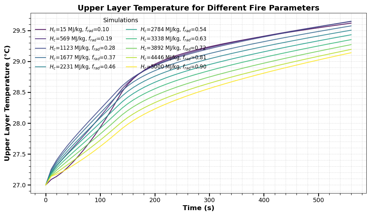
Step 5: Analyze Generated Data

Now we visualize our generated dataset to understand how the parameter variations affect fire behavior.

Each line represents a different combination of heat of combustion and radiative fraction values.

plt.figure(figsize=(12, 7))
colors = plt.get_cmap("viridis")(np.linspace(0, 1, len(all_runs)))

for idx, run in enumerate(all_runs):
    upper_layer = run["outputs"]["compartments"]["ULT_1"]
    time = run["outputs"]["compartments"]["Time"]
    plt.plot(
        time,
        upper_layer,
        label=(f"$H_c$={run['hoc']:.0f} MJ/kg, $f_{{rad}}$={run['rf']:.2f}"),
        linewidth=2,
        alpha=0.85,
        color=colors[idx],
    )

plt.xlabel("Time (s)", fontsize=16, fontweight="bold")
plt.ylabel("Upper Layer Temperature (°C)", fontsize=16, fontweight="bold")
plt.title(
    "Upper Layer Temperature for Different Fire Parameters",
    fontsize=18,
    fontweight="bold",
)
plt.legend(
    loc="upper left",
    fontsize=12,
    frameon=False,
    ncol=2,
    title="Simulations",
    title_fontsize=14,
)
plt.grid(True, which="both", linestyle="--", linewidth=0.7, alpha=0.5)
plt.minorticks_on()
plt.tick_params(axis="both", which="major", labelsize=14, length=7, width=2)
plt.tick_params(axis="both", which="minor", labelsize=12, length=4, width=1)
plt.tight_layout()
plt.show()

Cleanup

CFAST generates multiple output files during each simulation run.

files_removed = 0
for fname in os.listdir("."):
    if fname.startswith("data_gen_sim_"):
        try:
            os.remove(fname)
            files_removed += 1
        except Exception as e:
            print(f"Could not remove {fname}: {e}")

print(f"Cleanup complete. Removed {files_removed} simulation files.")

Cleanup complete. Removed 120 simulation files.