05 Operational research with optimization algorithms

This example demonstrates how to use optimization algorithms to find the best parameter values for CFAST fire simulations.

We’ll use SciPy’s optimization algorithms to efficiently explore the parameter space and find optimal fire model configurations.

Step 1: Import Required Libraries

We’ll import:

• NumPy: For generating parameter ranges and arrays

• Pandas: For organizing and analyzing simulation results

• Matplotlib: For visualizing the generated data

• SciPy: For optimization algorithms (see minimize)

• Scikit-learn: For parameter scaling and preprocessing (see MinMaxScaler)

• PyCFAST: For parsing and running CFAST models (see parse_cfast_file and run)

import matplotlib.pyplot as plt
import numpy as np
import pandas as pd
from scipy import optimize
from sklearn.preprocessing import MinMaxScaler

from pycfast.parsers import parse_cfast_file

Step 2: Load Base Model

We start with an existing CFAST model that will serve as our optimization baseline. This model contains all simulation settings and components.

For this example, we use parse_cfast_file to load the SP_AST_Diesel_1p1.in model which is fast to compute, making it suitable for optimization studies.

model = parse_cfast_file("data/SP_AST_Diesel_1p1.in")

The parsed model is displayed below.

print(model.summary())

Model: SP_AST_Diesel_1p1_parsed.in
Simulation: 'CFAST Simulation' (1800s)

Components:
  Material Properties (1):
    Material 'STEELSHT' (Steel Plain Carbon (1/16 in)): k=48.0, ρ=7854.0, c=0.559, t=0.0015, ε=0.9
  Compartment (1):
    Compartment 'Compartment 1': 100.0x100.0x100.0 m, volume: 1000000.00 m³ (ceiling: OFF, wall: OFF, floor: OFF)
  Wall Vents (4):
    Wall Vent 'WallVent_1': Compartment 1 ↔ OUTSIDE, 100.0x100.0 m, bottom: 0.0 m
    Wall Vent 'WallVent_2': Compartment 1 ↔ OUTSIDE, 100.0x100.0 m, bottom: 0.0 m
    Wall Vent 'WallVent_3': Compartment 1 ↔ OUTSIDE, 100.0x100.0 m, bottom: 0.0 m
    Wall Vent 'WallVent_4': Compartment 1 ↔ OUTSIDE, 100.0x100.0 m, bottom: 0.0 m
  Fire (1):
    Fire 'n-Decane Test 1' (n-Decane Test 1_Fire) in 'Compartment 1' at (50, 50) (peak: 2 kW, duration: 27min, χr: 0.35)
  Device (5):
    Target 'Targ 1' (PLATE) in 'Compartment 1' at (50, 50, 1.45) (material: STEELSHT, depth: 0.00075m)
    Target 'Targ 2' (PLATE) in 'Compartment 1' at (50, 50, 2.45) (material: STEELSHT, depth: 0.00075m)
    Target 'Targ 3' (PLATE) in 'Compartment 1' at (50, 50, 3.45) (material: STEELSHT, depth: 0.00075m)
    Target 'Targ 4' (PLATE) in 'Compartment 1' at (50, 50, 4.45) (material: STEELSHT, depth: 0.00075m)
    Target 'Targ 5' (PLATE) in 'Compartment 1' at (50, 50, 5.45) (material: STEELSHT, depth: 0.00075m)

Step 3: Define the Optimization Problem

We specify:

1. Parameters to optimize: Which model inputs to vary

2. Parameter bounds: Realistic ranges for each parameter

3. Starting point: Initial guess for the optimization

4. Objective: What to maximize/minimize (here: maximize TRGSURT_2 temperature)

Parameters chosen:

• Soot yield: Amount of soot produced by combustion (affects visibility and radiation)

• Radiative fraction: Portion of fire energy released as radiation (affects heat transfer)

We keep the problem simple with 2 parameters for demonstration, but you can optimize as many parameters as needed.

bounds = {
    "soot_yield": [0.01, 0.12],
    "radiative_fraction": [0.20, 0.45],
}

Initial guess (starting point) for optimization.

x0 = {"soot_yield": 0.05, "radiative_fraction": 0.35}

param_names = list(bounds.keys())

print("Optimization problem defined:")
for name, bound in bounds.items():
    print(f"{name}: [{bound[0]}, {bound[1]}]")

Optimization problem defined:
soot_yield: [0.01, 0.12]
radiative_fraction: [0.2, 0.45]

Step 4: Format Bounds for SciPy

We scale and prepare bounds in the format required by SciPy optimization functions.

bounds_array = np.array(list(bounds.values()))

Create scaler that will map from original bounds to [0,1] for each parameter

scaler = MinMaxScaler(feature_range=(0, 1))

scaler.fit(bounds_array.T)

scaled_bounds = [(0.0, 1.0) for _ in range(len(bounds))]
print(f"Scaled bounds: {scaled_bounds}")

x0_array = np.array(list(x0.values())).reshape(1, -1)
scaled_x0 = scaler.transform(x0_array).flatten()
print(f"Original x0: {list(x0.values())}")
print(f"Scaled x0: {scaled_x0}")

Scaled bounds: [(0.0, 1.0), (0.0, 1.0)]
Original x0: [0.05, 0.35]
Scaled x0: [0.36363636 0.6       ]

Step 5: Define Objective Function

The objective function is the heart of optimization. It:

• Receives scaled parameters from the optimizer

• Converts back to physical units using the scaler

• Runs the simulation with run

• Returns the negative temperature (since SciPy minimizes, but our goal is to maximize temperature)

optimization_path = []  # Track the actual optimization path


def objective_function(x):
    x = np.array([x])
    x = scaler.inverse_transform(x.reshape(1, -1))
    x = x.transpose()
    x = [x[0][0], x[1][0]]
    soot_yield = x[0]
    radiative_fraction = x[1]

    data_table = [
        row[:5] + [soot_yield] + row[6:] if len(row) > 6 else row
        for row in model.fires[0].data_table
    ]

    temp_model = model.update_fire_params(
        fire="n-Decane Test 1_Fire",
        data_table=data_table,
        radiative_fraction=radiative_fraction,
    )

    results = temp_model.run()

    max_trgsurt_2 = results["devices"]["TRGSURT_2"].max()
    print(
        f"Computing point: SY={soot_yield:.4f}, RF={radiative_fraction:.4f}, "
        f"Temp={max_trgsurt_2:.2f}"
    )

    optimization_path.append((soot_yield, radiative_fraction, max_trgsurt_2))

    return -max_trgsurt_2

Step 6: Generate Complete Function Map

Before optimization, we evaluate the objective function on a grid to visualize the landscape and validate optimizer results. This helps us understand if the function is smooth or has local minima. In practice, this step can be skipped for high-dimensional problems because of the curse of dimensionality, but for 2D or 3D problems it provides valuable insights.

grid_resolution = 15

soot_yield_grid = np.linspace(
    bounds["soot_yield"][0], bounds["soot_yield"][1], grid_resolution
)
radiative_fraction_grid = np.linspace(
    bounds["radiative_fraction"][0], bounds["radiative_fraction"][1], grid_resolution
)

function_map = {}
temperature_grid = np.zeros((grid_resolution, grid_resolution))

total_evaluations = grid_resolution * grid_resolution
evaluation_count = 0

for i, soot_yield in enumerate(soot_yield_grid):
    for j, radiative_fraction in enumerate(radiative_fraction_grid):
        evaluation_count += 1

        if evaluation_count % 25 == 0 or evaluation_count == total_evaluations:
            print(
                f"Progress: {evaluation_count}/{total_evaluations} ({100 * evaluation_count / total_evaluations:.1f}%)"
            )

        data_table = [
            row[:5] + [soot_yield] + row[6:] if len(row) > 6 else row
            for row in model.fires[0].data_table
        ]

        temp_model = model.update_fire_params(
            fire="n-Decane Test 1_Fire",
            data_table=data_table,
            radiative_fraction=radiative_fraction,
        )

        results = temp_model.run()

        max_trgsurt_2 = results["devices"]["TRGSURT_2"].max()

        function_map[(soot_yield, radiative_fraction)] = max_trgsurt_2
        temperature_grid[i, j] = max_trgsurt_2

SY_grid, RF_grid = np.meshgrid(soot_yield_grid, radiative_fraction_grid)

grid_df = pd.DataFrame(
    [(k[0], k[1], v) for k, v in function_map.items()],
    columns=["soot_yield", "radiative_fraction", "max_trgsurt_2"],
)

Progress: 25/225 (11.1%)
Progress: 50/225 (22.2%)
Progress: 75/225 (33.3%)
Progress: 100/225 (44.4%)
Progress: 125/225 (55.6%)
Progress: 150/225 (66.7%)
Progress: 175/225 (77.8%)
Progress: 200/225 (88.9%)
Progress: 225/225 (100.0%)

Statistics about the function map and default model performance for later comparison

default_max_temp = model.run()["devices"]["TRGSURT_2"].max()

print(f"Minimum temperature: {grid_df['max_trgsurt_2'].min():.2f} °C")
print(f"Maximum temperature: {grid_df['max_trgsurt_2'].max():.2f} °C")
print(f"Mean temperature: {grid_df['max_trgsurt_2'].mean():.2f} °C")
print(f"Default model temperature: {default_max_temp:.2f} °C")

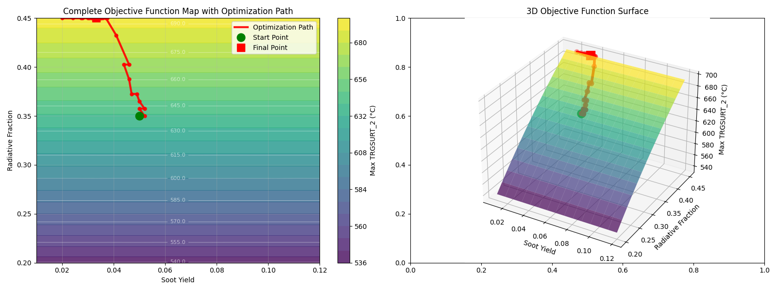
Minimum temperature: 539.51 °C
Maximum temperature: 693.05 °C
Mean temperature: 621.25 °C
Default model temperature: 639.11 °C

Step 7: Run Optimization Algorithm

Now we execute the Nelder-Mead optimization algorithm. This method requires no gradients, uses a simplex to converge toward the optimum, and respects parameter constraints during the search.

result = optimize.minimize(
    objective_function, x0=scaled_x0, method="Nelder-Mead", bounds=scaled_bounds
)

Computing point: SY=0.0500, RF=0.3500, Temp=639.11
Computing point: SY=0.0520, RF=0.3500, Temp=639.14
Computing point: SY=0.0500, RF=0.3575, Temp=643.46
Computing point: SY=0.0520, RF=0.3575, Temp=643.44
Computing point: SY=0.0500, RF=0.3650, Temp=647.73
Computing point: SY=0.0490, RF=0.3725, Temp=651.95
Computing point: SY=0.0470, RF=0.3725, Temp=651.95
Computing point: SY=0.0445, RF=0.3800, Temp=656.14
Computing point: SY=0.0435, RF=0.3950, Temp=664.36
Computing point: SY=0.0402, RF=0.4138, Temp=674.40
Computing point: SY=0.0357, RF=0.4213, Temp=678.35
Computing point: SY=0.0291, RF=0.4456, Temp=690.85
Computing point: SY=0.0249, RF=0.4500, Temp=693.00
Computing point: SY=0.0151, RF=0.4500, Temp=693.00
Computing point: SY=0.0100, RF=0.4500, Temp=693.01
Computing point: SY=0.0100, RF=0.4500, Temp=693.01
Computing point: SY=0.0100, RF=0.4500, Temp=693.01
Computing point: SY=0.0100, RF=0.4500, Temp=693.01
Computing point: SY=0.0100, RF=0.4500, Temp=693.01

Maximum temperature found by optimization (negate since we minimized the negative)

max_temp_found = -result.fun
print(f"{max_temp_found:.2f} °C")

693.01 °C

Optimized parameters in original units

optimized_params = dict(zip(param_names, result.x, strict=False))
print("Optimized parameters:")
for pname, pval in optimized_params.items():
    idx = list(param_names).index(pname)
    arr = np.zeros((1, len(param_names)))
    arr[0, idx] = pval
    unscaled_val = scaler.inverse_transform(arr)[0][idx]
    print(f"{pname}: {unscaled_val:.2f}")

Optimized parameters:
soot_yield: 0.01
radiative_fraction: 0.45

Step 8: Visualize Results

We visualize the complete function map with the optimization path overlaid to see how the optimizer navigated the landscape.

fig, (ax1, ax2) = plt.subplots(1, 2, figsize=(16, 6))

contour = ax1.contourf(
    SY_grid, RF_grid, temperature_grid.T, levels=20, cmap="viridis", alpha=0.8
)
contour_lines = ax1.contour(
    SY_grid,
    RF_grid,
    temperature_grid.T,
    levels=10,
    colors="white",
    alpha=0.6,
    linewidths=0.5,
)
ax1.clabel(contour_lines, inline=True, fontsize=8, fmt="%.1f")

if optimization_path:
    path_soot = [point[0] for point in optimization_path]
    path_rf = [point[1] for point in optimization_path]

    ax1.plot(
        path_soot, path_rf, "r-", linewidth=3, alpha=0.9, label="Optimization Path"
    )
    ax1.plot(path_soot, path_rf, "ro", markersize=5, alpha=0.9)

    ax1.plot(path_soot[0], path_rf[0], "go", markersize=12, label="Start Point")
    ax1.plot(path_soot[-1], path_rf[-1], "rs", markersize=12, label="Final Point")

ax1.set_xlabel("Soot Yield")
ax1.set_ylabel("Radiative Fraction")
ax1.set_title("Complete Objective Function Map with Optimization Path")
ax1.legend()
ax1.grid(True, alpha=0.3)
plt.colorbar(contour, ax=ax1, label="Max TRGSURT_2 (°C)")

ax2 = fig.add_subplot(122, projection="3d")
surface = ax2.plot_surface(
    SY_grid, RF_grid, temperature_grid.T, cmap="viridis", alpha=0.7
)

if optimization_path:
    path_temps = [point[2] for point in optimization_path]
    ax2.plot(
        path_soot, path_rf, path_temps, "r-", linewidth=4, label="Optimization Path"
    )
    ax2.scatter(path_soot, path_rf, path_temps, c="red", s=50)
    ax2.scatter(
        [path_soot[0]], [path_rf[0]], [path_temps[0]], c="green", s=150, label="Start"
    )
    ax2.scatter(
        [path_soot[-1]],
        [path_rf[-1]],
        [path_temps[-1]],
        c="red",
        s=150,
        marker="s",
        label="Final",
    )

ax2.set_xlabel("Soot Yield")
ax2.set_ylabel("Radiative Fraction")
ax2.set_zlabel("Max TRGSURT_2 (°C)")
ax2.set_title("3D Objective Function Surface")

plt.tight_layout()
plt.show()

Step 9: Analyze Optimization Performance

We compare the optimization results to the complete function map to understand how well the optimizer performed, how close it got to the global optimum, and how much improvement was achieved over the default model.

max_idx = np.unravel_index(np.argmax(temperature_grid), temperature_grid.shape)
global_opt_soot = soot_yield_grid[max_idx[0]]
global_opt_rf = radiative_fraction_grid[max_idx[1]]
global_opt_temp = temperature_grid[max_idx]

final_temp = optimization_path[-1][2]
path_temps = [point[2] for point in optimization_path]

dist_to_optimum = np.sqrt(
    (path_soot[-1] - global_opt_soot) ** 2 + (path_rf[-1] - global_opt_rf) ** 2
)

print("Function Map Statistics:")
print(
    f"Grid resolution: {grid_resolution}x{grid_resolution}"
    f" = {grid_resolution**2} points"
)
print(
    f"Temperature range: {grid_df['max_trgsurt_2'].min():.2f}"
    f" - {grid_df['max_trgsurt_2'].max():.2f} °C"
)
print(f"Temperature std dev: {grid_df['max_trgsurt_2'].std():.2f} °C")
print("\nGlobal Optimum (from complete map):")
print(f"Soot Yield: {global_opt_soot:.4f}")
print(f"Radiative Fraction: {global_opt_rf:.4f}")
print(f"Max Temperature: {global_opt_temp:.2f} °C")
print("\nOptimization Results:")
print(
    f"Start point: SY={path_soot[0]:.4f}, RF={path_rf[0]:.4f}, "
    f"Temp={path_temps[0]:.2f} °C"
)
print(
    f"Final point: SY={path_soot[-1]:.4f}, RF={path_rf[-1]:.4f}, "
    f"Temp={path_temps[-1]:.2f} °C"
)
print(f"Function evaluations: {len(optimization_path)}")
print(f"Temperature improvement: {path_temps[-1] - path_temps[0]:.2f} °C")
print(f"Distance from global optimum: {dist_to_optimum:.4f}")

improvement_achieved = path_temps[-1] - default_max_temp
max_possible_improvement = global_opt_temp - default_max_temp
efficiency = (
    (improvement_achieved / max_possible_improvement) * 100
    if max_possible_improvement > 0
    else 0
)
print(f"Optimization efficiency: {efficiency:.1f}% of maximum possible improvement")

Function Map Statistics:
Grid resolution: 15x15 = 225 points
Temperature range: 539.51 - 693.05 °C
Temperature std dev: 47.34 °C

Global Optimum (from complete map):
Soot Yield: 0.0414
Radiative Fraction: 0.4500
Max Temperature: 693.05 °C

Optimization Results:
Start point: SY=0.0500, RF=0.3500, Temp=639.11 °C
Final point: SY=0.0100, RF=0.4500, Temp=693.01 °C
Function evaluations: 19
Temperature improvement: 53.90 °C
Distance from global optimum: 0.0314
Optimization efficiency: 99.9% of maximum possible improvement

Additional visualizations to analyze optimization performance in detail

fig, ((ax1, ax2), (ax3, ax4)) = plt.subplots(2, 2, figsize=(15, 10))

iterations = range(1, len(optimization_path) + 1)
path_soot = [point[0] for point in optimization_path]
path_rf = [point[1] for point in optimization_path]
path_temps = [point[2] for point in optimization_path]

ax1.plot(
    iterations, path_temps, "b-o", linewidth=2, markersize=4, label="Optimization Path"
)
ax1.axhline(
    y=default_max_temp,
    color="r",
    linestyle="--",
    alpha=0.7,
    label=f"Default Model ({default_max_temp:.2f} °C)",
)
ax1.axhline(
    y=global_opt_temp,
    color="g",
    linestyle="--",
    alpha=0.7,
    label=f"Global Optimum ({global_opt_temp:.2f} °C)",
)
ax1.set_xlabel("Iteration")
ax1.set_ylabel("Max TRGSURT_2 (°C)")
ax1.set_title("Convergence History")
ax1.grid(True, alpha=0.3)
ax1.legend()

ax2.plot(iterations, path_soot, "g-o", linewidth=2, markersize=4, label="Soot Yield")
ax2.plot(
    iterations, path_rf, "m-s", linewidth=2, markersize=4, label="Radiative Fraction"
)
ax2.axhline(
    y=global_opt_soot, color="g", linestyle=":", alpha=0.7, label="Global Opt SY"
)
ax2.axhline(y=global_opt_rf, color="m", linestyle=":", alpha=0.7, label="Global Opt RF")
ax2.set_xlabel("Iteration")
ax2.set_ylabel("Parameter Value")
ax2.set_title("Parameter Evolution")
ax2.grid(True, alpha=0.3)
ax2.legend()

distances = [
    np.sqrt((sy - global_opt_soot) ** 2 + (rf - global_opt_rf) ** 2)
    for sy, rf in zip(path_soot, path_rf, strict=False)
]
ax3.plot(iterations, distances, "r-o", linewidth=2, markersize=4)
ax3.set_xlabel("Iteration")
ax3.set_ylabel("Distance from Global Optimum")
ax3.set_title("Convergence to Global Optimum")
ax3.grid(True, alpha=0.3)
ax3.set_yscale("log")

improvements = [temp - default_max_temp for temp in path_temps]
max_improvement = global_opt_temp - default_max_temp
efficiency = [
    (imp / max_improvement) * 100 if max_improvement > 0 else 0 for imp in improvements
]

ax4.plot(iterations, efficiency, "purple", linewidth=2, marker="o", markersize=4)
ax4.axhline(
    y=100, color="g", linestyle="--", alpha=0.7, label="100% Efficiency (Global Opt)"
)
ax4.set_xlabel("Iteration")
ax4.set_ylabel("Optimization Efficiency (%)")
ax4.set_title("Optimization Efficiency Over Time")
ax4.grid(True, alpha=0.3)
ax4.legend()
ax4.set_ylim(0, max(105, max(efficiency) * 1.1))

plt.tight_layout()
plt.show()

print(f"Initial efficiency: {efficiency[0]:.1f}%")
print(f"Final efficiency: {efficiency[-1]:.1f}%")
print(f"Best efficiency achieved: {max(efficiency):.1f}%")
print(f"Final distance from global optimum: {distances[-1]:.4f}")

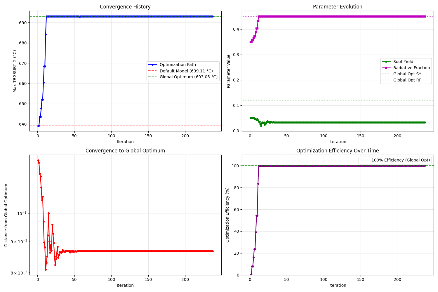
Initial efficiency: 0.0%
Final efficiency: 99.9%
Best efficiency achieved: 99.9%
Final distance from global optimum: 0.0314

Cleanup

import glob
import os

files_to_remove = glob.glob("SP_AST_Diesel_1p1*")

for file in files_to_remove:
    if os.path.exists(file):
        os.remove(file)
        print(f"Removed {file}")

if files_to_remove:
    print("Cleanup completed!")
else:
    print("No files to clean up.")

Removed SP_AST_Diesel_1p1_parsed.plt
Removed SP_AST_Diesel_1p1_parsed.in
Removed SP_AST_Diesel_1p1_parsed_zone.csv
Removed SP_AST_Diesel_1p1_parsed.smv
Removed SP_AST_Diesel_1p1_parsed_walls.csv
Removed SP_AST_Diesel_1p1_parsed_masses.csv
Removed SP_AST_Diesel_1p1_parsed.status
Removed SP_AST_Diesel_1p1_parsed.log
Removed SP_AST_Diesel_1p1_parsed.out
Removed SP_AST_Diesel_1p1_parsed_vents.csv
Removed SP_AST_Diesel_1p1_parsed_devices.csv
Removed SP_AST_Diesel_1p1_parsed_compartments.csv
Cleanup completed!